
|
Welcome to ShortScience.org! |


|
- ShortScience.org is a platform for post-publication discussion aiming to improve accessibility and reproducibility of research ideas.
- The website has 1584 public summaries, mostly in machine learning, written by the community and organized by paper, conference, and year.
- Reading summaries of papers is useful to obtain the perspective and insight of another reader, why they liked or disliked it, and their attempt to demystify complicated sections.
- Also, writing summaries is a good exercise to understand the content of a paper because you are forced to challenge your assumptions when explaining it.
- Finally, you can keep up to date with the flood of research by reading the latest summaries on our Twitter and Facebook pages.
Improving Transferability of Adversarial Examples with Input Diversity
Cihang Xie and Zhishuai Zhang and Yuyin Zhou and Song Bai and Jianyu Wang and Zhou Ren and Alan Yuille
arXiv e-Print archive - 2018 via Local arXiv
Keywords: cs.CV, cs.LG, stat.ML
First published: 2018/03/19 (6 years ago)
Abstract: Though CNNs have achieved the state-of-the-art performance on various vision tasks, they are vulnerable to adversarial examples --- crafted by adding human-imperceptible perturbations to clean images. However, most of the existing adversarial attacks only achieve relatively low success rates under the challenging black-box setting, where the attackers have no knowledge of the model structure and parameters. To this end, we propose to improve the transferability of adversarial examples by creating diverse input patterns. Instead of only using the original images to generate adversarial examples, our method applies random transformations to the input images at each iteration. Extensive experiments on ImageNet show that the proposed attack method can generate adversarial examples that transfer much better to different networks than existing baselines. By evaluating our method against top defense solutions and official baselines from NIPS 2017 adversarial competition, the enhanced attack reaches an average success rate of 73.0%, which outperforms the top-1 attack submission in the NIPS competition by a large margin of 6.6%. We hope that our proposed attack strategy can serve as a strong benchmark baseline for evaluating the robustness of networks to adversaries and the effectiveness of different defense methods in the future. Code is available at https://github.com/cihangxie/DI-2-FGSM.
more
less
Cihang Xie and Zhishuai Zhang and Yuyin Zhou and Song Bai and Jianyu Wang and Zhou Ren and Alan Yuille
arXiv e-Print archive - 2018 via Local arXiv
Keywords: cs.CV, cs.LG, stat.ML
First published: 2018/03/19 (6 years ago)
Abstract: Though CNNs have achieved the state-of-the-art performance on various vision tasks, they are vulnerable to adversarial examples --- crafted by adding human-imperceptible perturbations to clean images. However, most of the existing adversarial attacks only achieve relatively low success rates under the challenging black-box setting, where the attackers have no knowledge of the model structure and parameters. To this end, we propose to improve the transferability of adversarial examples by creating diverse input patterns. Instead of only using the original images to generate adversarial examples, our method applies random transformations to the input images at each iteration. Extensive experiments on ImageNet show that the proposed attack method can generate adversarial examples that transfer much better to different networks than existing baselines. By evaluating our method against top defense solutions and official baselines from NIPS 2017 adversarial competition, the enhanced attack reaches an average success rate of 73.0%, which outperforms the top-1 attack submission in the NIPS competition by a large margin of 6.6%. We hope that our proposed attack strategy can serve as a strong benchmark baseline for evaluating the robustness of networks to adversaries and the effectiveness of different defense methods in the future. Code is available at https://github.com/cihangxie/DI-2-FGSM.


[link]
Xie et al. propose to improve the transferability of adversarial examples by computing them based on transformed input images. In particular, they adapt I-FGSM such that, in each iteration, the update is computed on a transformed version of the current image with probability $p$. When, at the same time attacking an ensemble of networks, this is shown to improve transferability. Also find this summary at [davidstutz.de](https://davidstutz.de/category/reading/).  |

Batch Normalization: Accelerating Deep Network Training by Reducing Internal Covariate Shift
Ioffe, Sergey and Szegedy, Christian
International Conference on Machine Learning - 2015 via Local Bibsonomy
Keywords: dblp
Ioffe, Sergey and Szegedy, Christian
International Conference on Machine Learning - 2015 via Local Bibsonomy
Keywords: dblp
|
[link]
The main contribution of this paper is introducing a new transformation that the authors call Batch Normalization (BN). The need for BN comes from the fact that during the training of deep neural networks (DNNs) the distribution of each layer’s input change. This phenomenon is called internal covariate shift (ICS).

#### What is BN?
Normalize each (scalar) feature independently with respect to the mean and variance of the mini batch. Scale and shift the normalized values with two new parameters (per activation) that will be learned. The BN consists of making normalization part of the model architecture.

#### What do we gain?
According to the author, the use of BN provides a great speed up in the training of DNNs. In particular, the gains are greater when it is combined with higher learning rates. In addition, BN works as a regularizer for the model which allows to use less dropout or less L2 normalization. Furthermore, since the distribution of the inputs is normalized, it also allows to use sigmoids as activation functions without the saturation problem.

#### What follows?
This seems to be specially promising for training recurrent neural networks (RNNs). The vanishing and exploding gradient problems \cite{journals/tnn/BengioSF94} have their origin in the iteration of transformation that scale up or down the activations in certain directions (eigenvectors). It seems that this regularization would be specially useful in this context since this would allow the gradient to flow more easily. When we unroll the RNNs, we usually have ultra deep networks.

#### Like
* Simple idea that seems to improve training.
* Makes training faster.
* Simple to implement. Probably.
* You can be less careful with initialization.

#### Dislike
* Does not work with stochastic gradient descent (minibatch size = 1).
* This could reduce the parallelism of the algorithm since now all the examples in a mini batch are tied.
* Results on ensemble of networks for ImageNet makes it harder to evaluate the relevance of BN by itself. (Although they do mention the performance of a single model).
|

Bidirectional RNN for Medical Event Detection in Electronic Health Records
Jagannatha, Abhyuday N. and Yu, Hong
The Association for Computational Linguistics HLT-NAACL - 2016 via Local Bibsonomy
Keywords: dblp
Jagannatha, Abhyuday N. and Yu, Hong
The Association for Computational Linguistics HLT-NAACL - 2016 via Local Bibsonomy
Keywords: dblp
|
[link]
The authors have a dataset of 780 electronic health records and they use it to detect various medical events such as adverse drug events, drug dosage, etc. The task is done by assigning a label to each word in the document. https://i.imgur.com/bZ7yM0z.png Annotation statistics for the corpus of health records. They look at CRFs, LSTMs and GRUs. Both LSTMs and GRUs outperform the CRF, but the best performance is achieved by a GRU trained on whole documents. |

Do Deep Generative Models Know What They Don't Know?
Eric Nalisnick and Akihiro Matsukawa and Yee Whye Teh and Dilan Gorur and Balaji Lakshminarayanan
arXiv e-Print archive - 2018 via Local arXiv
Keywords: stat.ML, cs.LG
First published: 2018/10/22 (5 years ago)
Abstract: A neural network deployed in the wild may be asked to make predictions for inputs that were drawn from a different distribution than that of the training data. A plethora of work has demonstrated that it is easy to find or synthesize inputs for which a neural network is highly confident yet wrong. Generative models are widely viewed to be robust to such mistaken confidence as modeling the density of the input features can be used to detect novel, out-of-distribution inputs. In this paper we challenge this assumption. We find that the density learned by flow-based models, VAEs, and PixelCNNs cannot distinguish images of common objects such as dogs, trucks, and horses (i.e. CIFAR-10) from those of house numbers (i.e. SVHN), assigning a higher likelihood to the latter when the model is trained on the former. Moreover, we find evidence of this phenomenon when pairing several popular image data sets: FashionMNIST vs MNIST, CelebA vs SVHN, ImageNet vs CIFAR-10 / CIFAR-100 / SVHN. To investigate this curious behavior, we focus analysis on flow-based generative models in particular since they are trained and evaluated via the exact marginal likelihood. We find such behavior persists even when we restrict the flow models to constant-volume transformations. These transformations admit some theoretical analysis, and we show that the difference in likelihoods can be explained by the location and variances of the data and the model curvature. Our results caution against using the density estimates from deep generative models to identify inputs similar to the training distribution until their behavior for out-of-distribution inputs is better understood.
more
less
Eric Nalisnick and Akihiro Matsukawa and Yee Whye Teh and Dilan Gorur and Balaji Lakshminarayanan
arXiv e-Print archive - 2018 via Local arXiv
Keywords: stat.ML, cs.LG
First published: 2018/10/22 (5 years ago)
Abstract: A neural network deployed in the wild may be asked to make predictions for inputs that were drawn from a different distribution than that of the training data. A plethora of work has demonstrated that it is easy to find or synthesize inputs for which a neural network is highly confident yet wrong. Generative models are widely viewed to be robust to such mistaken confidence as modeling the density of the input features can be used to detect novel, out-of-distribution inputs. In this paper we challenge this assumption. We find that the density learned by flow-based models, VAEs, and PixelCNNs cannot distinguish images of common objects such as dogs, trucks, and horses (i.e. CIFAR-10) from those of house numbers (i.e. SVHN), assigning a higher likelihood to the latter when the model is trained on the former. Moreover, we find evidence of this phenomenon when pairing several popular image data sets: FashionMNIST vs MNIST, CelebA vs SVHN, ImageNet vs CIFAR-10 / CIFAR-100 / SVHN. To investigate this curious behavior, we focus analysis on flow-based generative models in particular since they are trained and evaluated via the exact marginal likelihood. We find such behavior persists even when we restrict the flow models to constant-volume transformations. These transformations admit some theoretical analysis, and we show that the difference in likelihoods can be explained by the location and variances of the data and the model curvature. Our results caution against using the density estimates from deep generative models to identify inputs similar to the training distribution until their behavior for out-of-distribution inputs is better understood.
|
[link]
CNNs predictions are known to be very sensitive to adversarial examples, which are samples generated to be wrongly classifiied with high confidence. On the other hand, probabilistic generative models such as `PixelCNN` and `VAEs` learn a distribution over the input domain hence could be used to detect ***out-of-distribution inputs***, e.g., by estimating their likelihood under the data distribution. This paper provides interesting results showing that distributions learned by generative models are not robust enough yet to employ them in this way.
  * **Pros (+):** convincing experiments on multiple generative models, more detailed analysis in the invertible flow case, interesting negative results.
  * **Cons (-):** It would be interesting to provide further results for different datasets / domain shifts to observe if this property can be quanitfied as a characteristics of the model or of the input data.


---

## Experimental negative result
Three classes of generative models are considered in this paper:
  * **Auto-regressive** models such as `PixelCNN` [1]
  * **Latent variable** models, such as `VAEs` [2]
  * Generative models with **invertible flows** [3], in particular `Glow` [4].

The authors train a generative model $G$ on input data $\mathcal X$ and then use it to evaluate the likelihood on both the training domain $\mathcal X$ and a different domain $\tilde{\mathcal X}$. Their main (negative) result is showing that **a model trained on the CIFAR-10 dataset yields a higher likelihood when evaluated on the SVHN test dataset than on the CIFAR-10 test (or even train) split**. Interestingly, the  converse, when training on SVHN and evaluating on CIFAR, is not true.

 This result was consistantly observed for various architectures including [1], [2] and [4], although it is of lesser effect in the `PixelCNN` case.

Intuitively, this could come from the fact that both of these datasets contain natural images and that CIFAR-10 is strictly more diverse than SVHN in terms of semantic content. Nonetheless, these datasets vastly differ in appearance, and this result is counter-intuitive as it goes against the direction that generative models can reliably be use to detect out-of-distribution samples. Furthermore, this observation also confirms the general idea that higher likelihoods does not necessarily coincide with better generated samples [5].

---
## Further analysis for invertible flow models
The authors further study this phenomenon in the invertible flow models case as they provide a more rigorous analytical framework (exact likelihood inference unlike VAE which only provide a bound on the true likelihood).

More specifically invertible flow models are characterized with a ***diffeomorphism*** (invertible function),  $f(x; \phi)$, between input space $\mathcal X$ and latent space $\mathcal Z$, and choice of the latent distribution $p(z; \psi)$. The ***change of variable formula*** links the density of $x$ and $z$ as follows:

$$
\int_x p_x(x)d_x = \int_x p_z(f(x)) \left| \frac{\partial f}{\partial x} \right| dx
$$


And the training objective under this transformation becomes

$$
\arg\max_{\theta} \log p_x(\mathbf{x}; \theta) = \arg\max_{\phi, \psi} \sum_i \log p_z(f(x_i; \phi); \psi) + \log \left| \frac{\partial f_{\phi}}{\partial x_i} \right|
$$

Typically, $p_z$ is chosen to be Gaussian, and samples are build by inverting $f$, i.e.,$z \sim p(\mathbf z),\  x = f^{-1}(z)$. And $f_{\phi}$ is build such that computing the log determinant of the Jacabian in the previous equation can be done efficiently.

First, they observe that contribution of the flow can be decomposed in a ***density*** element (left term) and a ***volume*** element (right term), resulting from the change of variables formula. Experiment results with Glow [4] show that the higher density  on SVHN mostly comes from the ***volume element contribution***.

Secondly, they try to directly analyze the difference in likelihood between two domains $\mathcal X$ and $\tilde{\mathcal X}$; which can be done by a second-order expansion of the log-likelihood locally around the expectation of the distribution (assuming $\mathbb{E} (\mathcal X) \sim \mathbb{E}(\tilde{\mathcal X})$). For the constant volume Glow module, the resulting analytical formula indeed confirms that the log-likelihood of SVHN should be higher than CIFAR's, as observed in practice.


  ---
## References
  * [1] Conditional Image Generation with PixelCNN Decoders, van den Oord et al, 2016
  * [2] Auto-Encoding Variational Bayes, Kingma and Welling, 2013
  * [3] Density estimation using Real NVP, Dinh et al., ICLR 2015
  * [4] Glow: Generative Flow with Invertible 1x1 Convolutions, Kingma and Dhariwal
  * [5] A Note on the Evaluation of Generative Models, Theis et al., ICLR 2016
|

Combining Markov Random Fields and Convolutional Neural Networks for Image Synthesis
Li, Chuan and Wand, Michael
Conference and Computer Vision and Pattern Recognition - 2016 via Local Bibsonomy
Keywords: dblp
Li, Chuan and Wand, Michael
Conference and Computer Vision and Pattern Recognition - 2016 via Local Bibsonomy
Keywords: dblp
|
[link]
* They describe a method that applies the style of a source image to a target image.
* Example: Let a normal photo look like a van Gogh painting.
* Example: Let a normal car look more like a specific luxury car.
* Their method builds upon the well known artistic style paper and uses a new MRF prior.
* The prior leads to locally more plausible patterns (e.g. less artifacts).
### How
* They reuse the content loss from the artistic style paper.
* The content loss was calculated by feed the source and target image through a network (here: VGG19) and then estimating the squared error of the euclidean distance between one or more hidden layer activations.
* They use layer `relu4_2` for the distance measurement.
* They replace the original style loss with a MRF based style loss.
* Step 1: Extract from the source image `k x k` sized overlapping patches.
* Step 2: Perform step (1) analogously for the target image.
* Step 3: Feed the source image patches through a pretrained network (here: VGG19) and select the representations `r_s` from specific hidden layers (here: `relu3_1`, `relu4_1`).
* Step 4: Perform step (3) analogously for the target image. (Result: `r_t`)
* Step 5: For each patch of `r_s` find the best matching patch in `r_t` (based on normalized cross correlation).
* Step 6: Calculate the sum of squared errors (based on euclidean distances) of each patch in `r_s` and its best match (according to step 5).
* They add a regularizer loss.
* The loss encourages smooth transitions in the synthesized image (i.e. few edges, corners).
* It is based on the raw pixel values of the last synthesized image.
* For each pixel in the synthesized image, they calculate the squared x-gradient and the squared y-gradient and then add both.
* They use the sum of all those values as their loss (i.e. `regularizer loss = <sum over all pixels> x-gradient^2 + y-gradient^2`).
* Their whole optimization problem is then roughly `image = argmin_image MRF-style-loss + alpha1 * content-loss + alpha2 * regularizer-loss`.
* In practice, they start their synthesis with a low resolution image and then progressively increase the resolution (each time performing some iterations of optimization).
* In practice, they sample patches from the style image under several different rotations and scalings.
### Results
* In comparison to the original artistic style paper:
* Less artifacts.
* Their method tends to preserve style better, but content worse.
* Can handle photorealistic style transfer better, so long as the images are similar enough. If no good matches between patches can be found, their method performs worse.
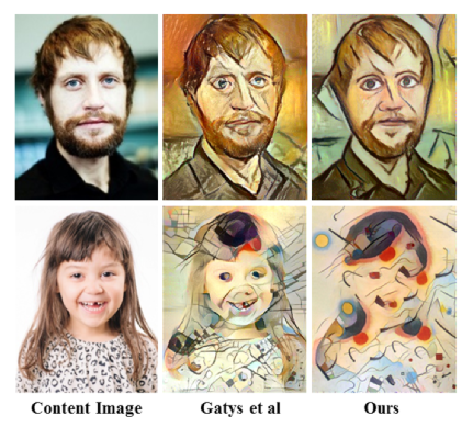
*Non-photorealistic example images. Their method vs. the one from the original artistic style paper.*
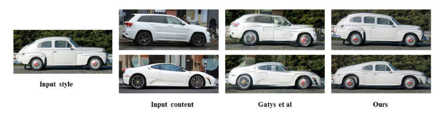
*Photorealistic example images. Their method vs. the one from the original artistic style paper.*
|
