
|
Welcome to ShortScience.org! |


|
- ShortScience.org is a platform for post-publication discussion aiming to improve accessibility and reproducibility of research ideas.
- The website has 1584 public summaries, mostly in machine learning, written by the community and organized by paper, conference, and year.
- Reading summaries of papers is useful to obtain the perspective and insight of another reader, why they liked or disliked it, and their attempt to demystify complicated sections.
- Also, writing summaries is a good exercise to understand the content of a paper because you are forced to challenge your assumptions when explaining it.
- Finally, you can keep up to date with the flood of research by reading the latest summaries on our Twitter and Facebook pages.
Batch Normalization: Accelerating Deep Network Training by Reducing Internal Covariate Shift
Ioffe, Sergey and Szegedy, Christian
International Conference on Machine Learning - 2015 via Local Bibsonomy
Keywords: dblp
Ioffe, Sergey and Szegedy, Christian
International Conference on Machine Learning - 2015 via Local Bibsonomy
Keywords: dblp


[link]
The main contribution of this paper is introducing a new transformation that the authors call Batch Normalization (BN). The need for BN comes from the fact that during the training of deep neural networks (DNNs) the distribution of each layer’s input change. This phenomenon is called internal covariate shift (ICS).

#### What is BN?
Normalize each (scalar) feature independently with respect to the mean and variance of the mini batch. Scale and shift the normalized values with two new parameters (per activation) that will be learned. The BN consists of making normalization part of the model architecture.

#### What do we gain?
According to the author, the use of BN provides a great speed up in the training of DNNs. In particular, the gains are greater when it is combined with higher learning rates. In addition, BN works as a regularizer for the model which allows to use less dropout or less L2 normalization. Furthermore, since the distribution of the inputs is normalized, it also allows to use sigmoids as activation functions without the saturation problem.

#### What follows?
This seems to be specially promising for training recurrent neural networks (RNNs). The vanishing and exploding gradient problems \cite{journals/tnn/BengioSF94} have their origin in the iteration of transformation that scale up or down the activations in certain directions (eigenvectors). It seems that this regularization would be specially useful in this context since this would allow the gradient to flow more easily. When we unroll the RNNs, we usually have ultra deep networks.

#### Like
* Simple idea that seems to improve training.
* Makes training faster.
* Simple to implement. Probably.
* You can be less careful with initialization.

#### Dislike
* Does not work with stochastic gradient descent (minibatch size = 1).
* This could reduce the parallelism of the algorithm since now all the examples in a mini batch are tied.
* Results on ensemble of networks for ImageNet makes it harder to evaluate the relevance of BN by itself. (Although they do mention the performance of a single model).
 |

Variational Information Maximisation for Intrinsically Motivated Reinforcement Learning
Mohamed, Shakir and Rezende, Danilo Jimenez
Neural Information Processing Systems Conference - 2015 via Local Bibsonomy
Keywords: dblp
Mohamed, Shakir and Rezende, Danilo Jimenez
Neural Information Processing Systems Conference - 2015 via Local Bibsonomy
Keywords: dblp
|
[link]
This paper presents a variational approach to the maximisation of mutual information in the context of a reinforcement learning agent. Mutual information in this context can provide a learning signal to the agent that is "intrinsically motivated", because it relies solely on the agent's state/beliefs and does not require from the ("outside") user an explicit definition of rewards.

Specifically, the learning objective, for a current state s, is the mutual information between the sequence of K actions a proposed by an exploration distribution $w(a|s)$ and the final state s' of the agent after performing these actions. To understand what the properties of this objective, it is useful to consider the form of this mutual information as a difference of conditional entropies:

$$I(a,s'|s) = H(a|s) - H(a|s',s)$$

Where $I(.|.)$ is the (conditional) mutual information and $H(.|.)$ is the (conditional) entropy. This objective thus asks that the agent find an exploration distribution that explores as much as possible (i.e. has high $H(a|s)$ entropy) but is such that these actions have predictable consequences (i.e. lead to predictable state s' so that $H(a|s',s)$ is low). So one could think of the agent as trying to learn to have control of as much of the environment as possible, thus this objective has also been coined as "empowerment".

The main contribution of this work is to show how to train, on a large scale (i.e. larger state space and action space) with this objective, using neural networks. They build on a variational lower bound on the mutual information and then derive from it a stochastic variational training algorithm for it. The procedure has 3 components: the exploration distribution $w(a|s)$, the environment $p(s'|s,a)$ (can be thought as an encoder, but which isn't modeled and is only interacted with/sampled from) and the planning model $p(a|s',s)$ (which is modeled and can be thought of as a decoder). The main technical contribution is in how to update the exploration distribution (see section 4.2.2 for the technical details).

This approach exploits neural networks of various forms. Neural autoregressive generative models are also used as models for the exploration distribution as well as the decoder or planning distribution. Interestingly, the framework allows to also learn the state representation s as a function of some "raw" representation x of states. For raw states corresponding to images (e.g. the pixels of the screen image in a game), CNNs are used.
|

Self-Normalizing Neural Networks
Günter Klambauer and Thomas Unterthiner and Andreas Mayr and Sepp Hochreiter
arXiv e-Print archive - 2017 via Local arXiv
Keywords: cs.LG, stat.ML
First published: 2017/06/08 (6 years ago)
Abstract: Deep Learning has revolutionized vision via convolutional neural networks (CNNs) and natural language processing via recurrent neural networks (RNNs). However, success stories of Deep Learning with standard feed-forward neural networks (FNNs) are rare. FNNs that perform well are typically shallow and, therefore cannot exploit many levels of abstract representations. We introduce self-normalizing neural networks (SNNs) to enable high-level abstract representations. While batch normalization requires explicit normalization, neuron activations of SNNs automatically converge towards zero mean and unit variance. The activation function of SNNs are "scaled exponential linear units" (SELUs), which induce self-normalizing properties. Using the Banach fixed-point theorem, we prove that activations close to zero mean and unit variance that are propagated through many network layers will converge towards zero mean and unit variance -- even under the presence of noise and perturbations. This convergence property of SNNs allows to (1) train deep networks with many layers, (2) employ strong regularization, and (3) to make learning highly robust. Furthermore, for activations not close to unit variance, we prove an upper and lower bound on the variance, thus, vanishing and exploding gradients are impossible. We compared SNNs on (a) 121 tasks from the UCI machine learning repository, on (b) drug discovery benchmarks, and on (c) astronomy tasks with standard FNNs and other machine learning methods such as random forests and support vector machines. SNNs significantly outperformed all competing FNN methods at 121 UCI tasks, outperformed all competing methods at the Tox21 dataset, and set a new record at an astronomy data set. The winning SNN architectures are often very deep. Implementations are available at: github.com/bioinf-jku/SNNs.
more
less
Günter Klambauer and Thomas Unterthiner and Andreas Mayr and Sepp Hochreiter
arXiv e-Print archive - 2017 via Local arXiv
Keywords: cs.LG, stat.ML
First published: 2017/06/08 (6 years ago)
Abstract: Deep Learning has revolutionized vision via convolutional neural networks (CNNs) and natural language processing via recurrent neural networks (RNNs). However, success stories of Deep Learning with standard feed-forward neural networks (FNNs) are rare. FNNs that perform well are typically shallow and, therefore cannot exploit many levels of abstract representations. We introduce self-normalizing neural networks (SNNs) to enable high-level abstract representations. While batch normalization requires explicit normalization, neuron activations of SNNs automatically converge towards zero mean and unit variance. The activation function of SNNs are "scaled exponential linear units" (SELUs), which induce self-normalizing properties. Using the Banach fixed-point theorem, we prove that activations close to zero mean and unit variance that are propagated through many network layers will converge towards zero mean and unit variance -- even under the presence of noise and perturbations. This convergence property of SNNs allows to (1) train deep networks with many layers, (2) employ strong regularization, and (3) to make learning highly robust. Furthermore, for activations not close to unit variance, we prove an upper and lower bound on the variance, thus, vanishing and exploding gradients are impossible. We compared SNNs on (a) 121 tasks from the UCI machine learning repository, on (b) drug discovery benchmarks, and on (c) astronomy tasks with standard FNNs and other machine learning methods such as random forests and support vector machines. SNNs significantly outperformed all competing FNN methods at 121 UCI tasks, outperformed all competing methods at the Tox21 dataset, and set a new record at an astronomy data set. The winning SNN architectures are often very deep. Implementations are available at: github.com/bioinf-jku/SNNs.
|
[link]
_Objective:_ Design Feed-Forward Neural Network (fully connected) that can be trained even with very deep architectures.
* _Dataset:_ [MNIST](yann.lecun.com/exdb/mnist/), [CIFAR10](https://www.cs.toronto.edu/%7Ekriz/cifar.html), [Tox21](https://tripod.nih.gov/tox21/challenge/) and [UCI tasks](https://archive.ics.uci.edu/ml/datasets/optical+recognition+of+handwritten+digits).
* _Code:_ [here](https://github.com/bioinf-jku/SNNs)
## Inner-workings:
They introduce a new activation functio the Scaled Exponential Linear Unit (SELU) which has the nice property of making neuron activations converge to a fixed point with zero-mean and unit-variance.
They also demonstrate that upper and lower bounds and the variance and mean for very mild conditions which basically means that there will be no exploding or vanishing gradients.
The activation function is:
[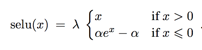](https://user-images.githubusercontent.com/17261080/27125901-1a4f7276-50f6-11e7-857d-ebad1ac94789.png)
With specific parameters for alpha and lambda to ensure the previous properties. The tensorflow impementation is:
def selu(x):
alpha = 1.6732632423543772848170429916717
scale = 1.0507009873554804934193349852946
return scale*np.where(x>=0.0, x, alpha*np.exp(x)-alpha)
They also introduce a new dropout (alpha-dropout) to compensate for the fact that [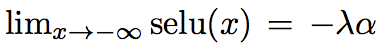](https://user-images.githubusercontent.com/17261080/27126174-e67d212c-50f6-11e7-8952-acad98b850be.png)
## Results:
Batch norm becomes obsolete and they are also able to train deeper architectures. This becomes a good choice to replace shallow architectures where random forest or SVM used to be the best results. They outperform most other techniques on small datasets.
[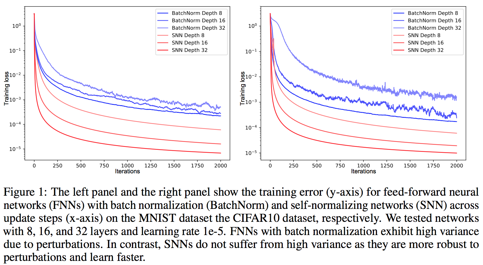](https://user-images.githubusercontent.com/17261080/27125798-bd04c256-50f5-11e7-8a74-b3b6a3fe82ee.png)
Might become a new standard for fully-connected activations in the future.
|

Improving Transferability of Adversarial Examples with Input Diversity
Cihang Xie and Zhishuai Zhang and Yuyin Zhou and Song Bai and Jianyu Wang and Zhou Ren and Alan Yuille
arXiv e-Print archive - 2018 via Local arXiv
Keywords: cs.CV, cs.LG, stat.ML
First published: 2018/03/19 (6 years ago)
Abstract: Though CNNs have achieved the state-of-the-art performance on various vision tasks, they are vulnerable to adversarial examples --- crafted by adding human-imperceptible perturbations to clean images. However, most of the existing adversarial attacks only achieve relatively low success rates under the challenging black-box setting, where the attackers have no knowledge of the model structure and parameters. To this end, we propose to improve the transferability of adversarial examples by creating diverse input patterns. Instead of only using the original images to generate adversarial examples, our method applies random transformations to the input images at each iteration. Extensive experiments on ImageNet show that the proposed attack method can generate adversarial examples that transfer much better to different networks than existing baselines. By evaluating our method against top defense solutions and official baselines from NIPS 2017 adversarial competition, the enhanced attack reaches an average success rate of 73.0%, which outperforms the top-1 attack submission in the NIPS competition by a large margin of 6.6%. We hope that our proposed attack strategy can serve as a strong benchmark baseline for evaluating the robustness of networks to adversaries and the effectiveness of different defense methods in the future. Code is available at https://github.com/cihangxie/DI-2-FGSM.
more
less
Cihang Xie and Zhishuai Zhang and Yuyin Zhou and Song Bai and Jianyu Wang and Zhou Ren and Alan Yuille
arXiv e-Print archive - 2018 via Local arXiv
Keywords: cs.CV, cs.LG, stat.ML
First published: 2018/03/19 (6 years ago)
Abstract: Though CNNs have achieved the state-of-the-art performance on various vision tasks, they are vulnerable to adversarial examples --- crafted by adding human-imperceptible perturbations to clean images. However, most of the existing adversarial attacks only achieve relatively low success rates under the challenging black-box setting, where the attackers have no knowledge of the model structure and parameters. To this end, we propose to improve the transferability of adversarial examples by creating diverse input patterns. Instead of only using the original images to generate adversarial examples, our method applies random transformations to the input images at each iteration. Extensive experiments on ImageNet show that the proposed attack method can generate adversarial examples that transfer much better to different networks than existing baselines. By evaluating our method against top defense solutions and official baselines from NIPS 2017 adversarial competition, the enhanced attack reaches an average success rate of 73.0%, which outperforms the top-1 attack submission in the NIPS competition by a large margin of 6.6%. We hope that our proposed attack strategy can serve as a strong benchmark baseline for evaluating the robustness of networks to adversaries and the effectiveness of different defense methods in the future. Code is available at https://github.com/cihangxie/DI-2-FGSM.
|
[link]
Xie et al. propose to improve the transferability of adversarial examples by computing them based on transformed input images. In particular, they adapt I-FGSM such that, in each iteration, the update is computed on a transformed version of the current image with probability $p$. When, at the same time attacking an ensemble of networks, this is shown to improve transferability. Also find this summary at [davidstutz.de](https://davidstutz.de/category/reading/). |

Better-than-Demonstrator Imitation Learning via Automatically-Ranked Demonstrations
Daniel S. Brown and Wonjoon Goo and Scott Niekum
arXiv e-Print archive - 2019 via Local arXiv
Keywords: cs.LG, stat.ML
First published: 2019/07/09 (4 years ago)
Abstract: The performance of imitation learning is typically upper-bounded by the performance of the demonstrator. While recent empirical results demonstrate that ranked demonstrations allow for better-than-demonstrator performance, preferences over demonstrations may be difficult to obtain, and little is known theoretically about when such methods can be expected to successfully extrapolate beyond the performance of the demonstrator. To address these issues, we first contribute a sufficient condition for better-than-demonstrator imitation learning and provide theoretical results showing why preferences over demonstrations can better reduce reward function ambiguity when performing inverse reinforcement learning. Building on this theory, we introduce Disturbance-based Reward Extrapolation (D-REX), a ranking-based imitation learning method that injects noise into a policy learned through behavioral cloning to automatically generate ranked demonstrations. These ranked demonstrations are used to efficiently learn a reward function that can then be optimized using reinforcement learning. We empirically validate our approach on simulated robot and Atari imitation learning benchmarks and show that D-REX outperforms standard imitation learning approaches and can significantly surpass the performance of the demonstrator. D-REX is the first imitation learning approach to achieve significant extrapolation beyond the demonstrator's performance without additional side-information or supervision, such as rewards or human preferences. By generating rankings automatically, we show that preference-based inverse reinforcement learning can be applied in traditional imitation learning settings where only unlabeled demonstrations are available.
more
less
Daniel S. Brown and Wonjoon Goo and Scott Niekum
arXiv e-Print archive - 2019 via Local arXiv
Keywords: cs.LG, stat.ML
First published: 2019/07/09 (4 years ago)
Abstract: The performance of imitation learning is typically upper-bounded by the performance of the demonstrator. While recent empirical results demonstrate that ranked demonstrations allow for better-than-demonstrator performance, preferences over demonstrations may be difficult to obtain, and little is known theoretically about when such methods can be expected to successfully extrapolate beyond the performance of the demonstrator. To address these issues, we first contribute a sufficient condition for better-than-demonstrator imitation learning and provide theoretical results showing why preferences over demonstrations can better reduce reward function ambiguity when performing inverse reinforcement learning. Building on this theory, we introduce Disturbance-based Reward Extrapolation (D-REX), a ranking-based imitation learning method that injects noise into a policy learned through behavioral cloning to automatically generate ranked demonstrations. These ranked demonstrations are used to efficiently learn a reward function that can then be optimized using reinforcement learning. We empirically validate our approach on simulated robot and Atari imitation learning benchmarks and show that D-REX outperforms standard imitation learning approaches and can significantly surpass the performance of the demonstrator. D-REX is the first imitation learning approach to achieve significant extrapolation beyond the demonstrator's performance without additional side-information or supervision, such as rewards or human preferences. By generating rankings automatically, we show that preference-based inverse reinforcement learning can be applied in traditional imitation learning settings where only unlabeled demonstrations are available.
|
[link]
## General Framework Extends T-REX (see [summary](https://www.shortscience.org/paper?bibtexKey=journals/corr/1904.06387&a=muntermulehitch)) so that preferences (rankings) over demonstrations are generated automatically (back to the common IL/IRL setting where we only have access to a set of unlabeled demonstrations). Also derives some theoretical requirements and guarantees for better-than-demonstrator performance. ## Motivations * Preferences over demonstrations may be difficult to obtain in practice. * There is no theoretical understanding of the requirements that lead to outperforming demonstrator. ## Contributions * Theoretical results (with linear reward function) on when better-than-demonstrator performance is possible: 1- the demonstrator must be suboptimal (room for improvement, obviously), 2- the learned reward must be close enough to the reward that the demonstrator is suboptimally optimizing for (be able to accurately capture the intent of the demonstrator), 3- the learned policy (optimal wrt the learned reward) must be close enough to the optimal policy (wrt to the ground truth reward). Obviously if we have 2- and a good enough RL algorithm we should have 3-, so it might be interesting to see if one can derive a requirement from only 1- and 2- (and possibly a good enough RL algo). * Theoretical results (with linear reward function) showing that pairwise preferences over demonstrations reduce the error and ambiguity of the reward learning. They show that without rankings two policies might have equal performance under a learned reward (that makes expert's demonstrations optimal) but very different performance under the true reward (that makes the expert optimal everywhere). Indeed, the expert's demonstration may reveal very little information about the reward of (suboptimal or not) unseen regions which may hurt very much the generalizations (even with RL as it would try to generalize to new states under a totally wrong reward). They also show that pairwise preferences over trajectories effectively give half-space constraints on the feasible reward function domain and thus may decrease exponentially the reward function ambiguity. * Propose a practical way to generate as many ranked demos as desired. ## Additional Assumption Very mild, assumes that a Behavioral Cloning (BC) policy trained on the provided demonstrations is better than a uniform random policy. ## Disturbance-based Reward Extrapolation (D-REX)   They also show that the more noise added to the BC policy the lower the performance of the generated trajs. ## Results Pretty much like T-REX. |
