* Usually GANs transform a noise vector `z` into images. `z` might be sampled from a normal or uniform distribution.
  * The effect of this is, that the components in `z` are deeply entangled.
    * Changing single components has hardly any influence on the generated images. One has to change multiple components to affect the image.
    * The components end up not being interpretable. Ideally one would like to have meaningful components, e.g. for human faces one that controls the hair length and a categorical one that controls the eye color.
  * They suggest a change to GANs based on Mutual Information, which leads to interpretable components.
    * E.g. for MNIST a component that controls the stroke thickness and a categorical component that controls the digit identity (1, 2, 3, ...).
    * These components are learned in a (mostly) unsupervised fashion.

### How
  * The latent code `c`
    * "Normal" GANs parameterize the generator as `G(z)`, i.e. G receives a noise vector and transforms it into an image.
    * This is changed to `G(z, c)`, i.e. G now receives a noise vector `z` and a latent code `c` and transforms both into an image.
    * `c` can contain multiple variables following different distributions, e.g. in MNIST a categorical variable for the digit identity and a gaussian one for the stroke thickness.
  * Mutual Information
    * If using a latent code via `G(z, c)`, nothing forces the generator to actually use `c`. It can easily ignore it and just deteriorate to `G(z)`.
    * To prevent that, they force G to generate images `x` in a way that `c` must be recoverable. So, if you have an image `x` you must be able to reliable tell which latent code `c` it has, which means that G must use `c` in a meaningful way.
    * This relationship can be expressed with mutual information, i.e. the mutual information between `x` and `c` must be high.
      * The mutual information between two variables X and Y is defined as `I(X; Y) = entropy(X) - entropy(X|Y) = entropy(Y) - entropy(Y|X)`.
      * If the mutual information between X and Y is high, then knowing Y helps you to decently predict the value of X (and the other way round).
      * If the mutual information between X and Y is low, then knowing Y doesn't tell you much about the value of X (and the other way round).
    * The new GAN loss becomes `old loss - lambda * I(G(z, c); c)`, i.e. the higher the mutual information, the lower the result of the loss function.
  * Variational Mutual Information Maximization
    * In order to minimize `I(G(z, c); c)`, one has to know the distribution `P(c|x)` (from image to latent code), which however is unknown.
    * So instead they create `Q(c|x)`, which is an approximation of `P(c|x)`.
    * `I(G(z, c); c)` is then computed using a lower bound maximization, similar to the one in variational autoencoders (called "Variational Information Maximization", hence the name "InfoGAN").
    * Basic equation: `LowerBoundOfMutualInformation(G, Q) = E[log Q(c|x)] + H(c) <= I(G(z, c); c)`
      * `c` is the latent code.
      * `x` is the generated image.
      * `H(c)` is the entropy of the latent codes (constant throughout the optimization).
      * Optimization w.r.t. Q is done directly.
      * Optimization w.r.t. G is done via the reparameterization trick.
    * If `Q(c|x)` approximates `P(c|x)` *perfectly*, the lower bound becomes the mutual information ("the lower bound becomes tight").
    * In practice, `Q(c|x)` is implemented as a neural network. Both Q and D have to process the generated images, which means that they can share many convolutional layers, significantly reducing the extra cost of training Q.

### Results
  * MNIST
    * They use for `c` one categorical variable (10 values) and two continuous ones (uniform between -1 and +1).
    * InfoGAN learns to associate the categorical one with the digit identity and the continuous ones with rotation and width.
    * Applying Q(c|x) to an image and then classifying only on the categorical variable (i.e. fully unsupervised) yields 95% accuracy.
    * Sampling new images with exaggerated continuous variables in the range `[-2,+2]` yields sound images (i.e. the network generalizes well).
    * ![MNIST examples](https://raw.githubusercontent.com/aleju/papers/master/neural-nets/images/InfoGAN__mnist.png?raw=true "MNIST examples")
  * 3D face images
    * InfoGAN learns to represent the faces via pose, elevation, lighting.
    * They used five uniform variables for `c`. (So two of them apparently weren't associated with anything sensible? They are not mentioned.)
  * 3D chair images
    * InfoGAN learns to represent the chairs via identity (categorical) and rotation or width (apparently they did two experiments).
    * They used one categorical variable (four values) and one continuous variable (uniform `[-1, +1]`).
  * SVHN
    * InfoGAN learns to represent lighting and to spot the center digit.
    * They used four categorical variables (10 values each) and two continuous variables (uniform `[-1, +1]`). (Again, a few variables were apparently not associated with anything sensible?)
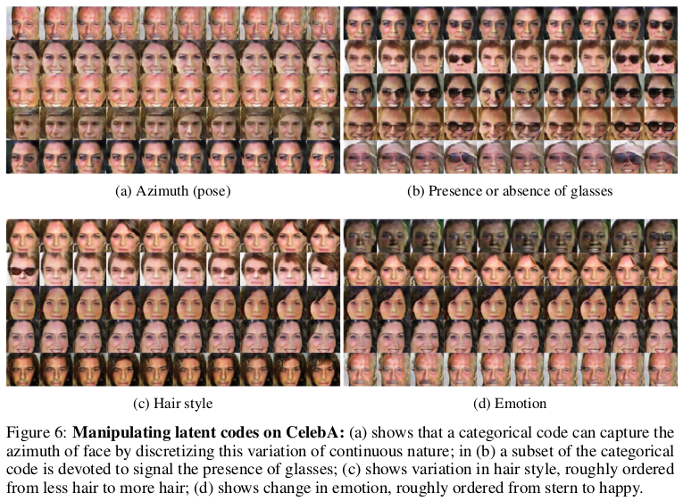
  * CelebA
    * InfoGAN learns to represent pose, presence of sunglasses (not perfectly), hair style and emotion (in the sense of "smiling or not smiling").
    * They used 10 categorical variables (10 values each). (Again, a few variables were apparently not associated with anything sensible?)
    * ![CelebA examples](https://raw.githubusercontent.com/aleju/papers/master/neural-nets/images/InfoGAN__celeba.png?raw=true "CelebA examples")

Fawzi et al. study robustness in the transition from random samples to semi-random and adversarial  samples. Specifically they present bounds relating the norm of an adversarial perturbation to the norm of random perturbations – for the exact form I refer to the paper. Personally, I find the definition of semi-random noise most interesting, as it allows to get an intuition for distinguishing random noise from adversarial examples. As in related literature, adversarial examples are defined as

$r_S(x_0) = \arg\min_{x_0 \in S} \|r\|_2$ s.t. $f(x_0 + r) \neq f(x_0)$

where $f$ is the classifier to attack and $S$ the set of allowed perturbations (e.g. requiring that the perturbed samples are still images). If $S$ is mostly unconstrained regarding the direction of $r$ in high dimensional space, Fawzi et al. consider $r$ to be an adversarial examples – intuitively, and adversary can choose $r$ arbitrarily to fool the classifier. If, however, the directions considered in $S$ are constrained to an $m$-dimensional subspace, Fawzi et al. consider $r$ to be semi-random noise. In the extreme case, if $m = 1$, $r$ is random noise. In this case, we can intuitively think of $S$ as a randomly chosen one dimensional subspace – i.e. a random direction in multi-dimensional space.

Also find this summary at [davidstutz.de](https://davidstutz.de/category/reading/).

Mask RCNN takes off from where Faster RCNN left, with some augmentations aimed at bettering instance segmentation (which was out of scope for FRCNN). Instance segmentation was achieved remarkably well in *DeepMask* , *SharpMask* and later *Feature Pyramid Networks* (FPN).

Faster RCNN was not designed for pixel-to-pixel alignment between network inputs and outputs. This is most evident in how RoIPool , the de facto core operation for attending to instances, performs coarse spatial quantization for feature extraction. Mask RCNN fixes that by introducing RoIAlign in place of RoIPool.

#### Methodology

Mask RCNN retains most of the architecture of Faster RCNN. It adds the a third branch for segmentation. The third branch takes the output from RoIAlign layer and predicts binary class masks for each class.

##### Major Changes and intutions

**Mask prediction**

Mask prediction segmentation predicts a binary mask for each RoI using fully convolution - and the stark difference being usage of *sigmoid* activation for predicting final mask instead of *softmax*, implies masks don't compete with each other. This *decouples* segmentation from classification. The class prediction branch is used for class prediction and for calculating loss, the mask of predicted loss is used calculating Lmask.

Also, they show that a single class agnostic mask prediction works almost as effective as separate mask for each class, thereby supporting their method of decoupling classification from segmentation

**RoIAlign**

RoIPool first quantizes a floating-number RoI to the discrete granularity of the feature map, this quantized RoI is then subdivided into spatial bins which are themselves quantized, and finally feature values covered by each bin are aggregated (usually by max pooling). Instead of  quantization of the RoI boundaries
or bin bilinear interpolation is used to compute the exact values of the input features at four regularly sampled locations in each RoI bin, and aggregate the result (using max or average).

**Backbone architecture**

Faster RCNN uses a VGG like structure for extracting features from image, weights of which were shared among RPN and region detection layers. Herein, authors experiment with 2 backbone architectures - ResNet based VGG like in FRCNN and ResNet based [FPN](http://www.shortscience.org/paper?bibtexKey=journals/corr/LinDGHHB16) based. FPN uses convolution feature maps from previous layers and recombining them to produce pyramid of feature maps to be used for prediction instead of single-scale feature layer (final output of conv layer before connecting to fc layers was used in Faster RCNN) 

**Training Objective**

The training objective looks like this 
![](https://i.imgur.com/snUq73Q.png)

Lmask is the addition from Faster RCNN. The method to calculate was mentioned above

#### Observation

Mask RCNN performs significantly better than COCO instance segmentation winners *without any bells and whiskers*. Detailed results are available in the paper

In this paper, the authors raise a very important point for instance based image retrieval. For a task like an image recognition features extracted from higher layer of deep networks works really well in general, but for task like instance based image retrieval features extracted from higher layers don't prove to be that useful, so the authors suggest that we take features from lower layer and on those features, apply [VLAD encoding](https://www.robots.ox.ac.uk/~vgg/publications/2013/arandjelovic13/arandjelovic13.pdf). On top of the VLAD encoding as part of post processing, we perform steps like intra-normalisation and then apply PCA and reduce the encoding to a size of 128 Dimension. The authors have performed their experiments using [Googlenet](https://www.cs.unc.edu/~wliu/papers/GoogLeNet.pdf) and [VGG-16](https://arxiv.org/pdf/1409.1556v6.pdf), and they tried Inception 3a, Inception 4a and Inception 4e on GoogleNet and conv4_2, conv5_1 and conv5_2 on VGG-16. The above mentioned layers has almost similar performance on the dataset they have used. The performance metric used by the authors is Mean Average Precision(MAP). 

This paper introduced Dropout, a new layer type. It has a parameter $\alpha \in (0, 1)$. The output dimensionality of a dropout layer is equal to its input dimensionality. With a probability of $\alpha$ any neurons output is set to 0. At testing time, the output of all neurons is multiplied with $\alpha$ to compensate for the fact that no output is set to 0.

A much better paper, by the same authors but 2 years later, is [Dropout: a simple way to prevent neural networks from overfitting](http://www.shortscience.org/paper?bibtexKey=journals/jmlr/SrivastavaHKSS14).

Dropout can be interpreted as training an ensemble of many networks, which share weights.

It was notably used by [ImageNet Classification with Deep Convolutional Neural Networks](http://www.shortscience.org/paper?bibtexKey=krizhevsky2012imagenet).