
|
Welcome to ShortScience.org! |


|
- ShortScience.org is a platform for post-publication discussion aiming to improve accessibility and reproducibility of research ideas.
- The website has 1584 public summaries, mostly in machine learning, written by the community and organized by paper, conference, and year.
- Reading summaries of papers is useful to obtain the perspective and insight of another reader, why they liked or disliked it, and their attempt to demystify complicated sections.
- Also, writing summaries is a good exercise to understand the content of a paper because you are forced to challenge your assumptions when explaining it.
- Finally, you can keep up to date with the flood of research by reading the latest summaries on our Twitter and Facebook pages.
Question Answering with Subgraph Embeddings
Antoine Bordes and Sumit Chopra and Jason Weston
arXiv e-Print archive - 2014 via Local arXiv
Keywords: cs.CL
First published: 2014/06/14 (9 years ago)
Abstract: This paper presents a system which learns to answer questions on a broad range of topics from a knowledge base using few hand-crafted features. Our model learns low-dimensional embeddings of words and knowledge base constituents; these representations are used to score natural language questions against candidate answers. Training our system using pairs of questions and structured representations of their answers, and pairs of question paraphrases, yields competitive results on a competitive benchmark of the literature.
more
less
Antoine Bordes and Sumit Chopra and Jason Weston
arXiv e-Print archive - 2014 via Local arXiv
Keywords: cs.CL
First published: 2014/06/14 (9 years ago)
Abstract: This paper presents a system which learns to answer questions on a broad range of topics from a knowledge base using few hand-crafted features. Our model learns low-dimensional embeddings of words and knowledge base constituents; these representations are used to score natural language questions against candidate answers. Training our system using pairs of questions and structured representations of their answers, and pairs of question paraphrases, yields competitive results on a competitive benchmark of the literature.


[link]
#### Introduction

* Open-domain Question Answering (Open QA) - efficiently querying large-scale knowledge base(KB) using natural language.
* Two main approaches:
    * Information Retrieval
        * Transform question (in natural language) into a valid query(in terms of KB) to get a broad set of candidate answers.
        * Perform fine-grained detection on candidate answers.
    * Semantic Parsing
        * Interpret the correct meaning of the question and convert it into an exact query.
* Limitations:
    * Human intervention to create lexicon, grammar, and schema.
* This work builds upon the previous work where an embedding model learns low dimensional vector representation of words and symbols.
* [Link](https://arxiv.org/abs/1406.3676) to the paper.

#### Task Definition

* Input - Training set of questions (paired with answers).
* KB providing a structure among the answers.
* Answers are entities in KB and questions are strings with one identified KB entity.
* The paper has used FREEBASE as the KB.
* Datasets
    * WebQuestions - Built using FREEBASE, Google Suggest API, and Mechanical Turk.
    * FREEBASE triplets transformed into questions.
    * Clue Web Extractions dataset with entities linked with FREEBASE triplets.
    * Dataset of paraphrased questions using WIKIANSWERS.

#### Embedding Questions and Answers

* Model learns low-dimensional vector embeddings of words in question entities and relation types of FREEBASE such that questions and their answers are represented close to each other in the joint embedding space.
* Scoring function $S(q, a)$, where $q$ is a question and $a$ is an answer, generates high score if $a$ answers $q$.
    * $S(q, a) = f(q)^{T} . g(a)$
    * $f(q)$ maps question to embedding space.
    * $f(q) = W \phi (q)$
    * $W$ is a matrix of dimension $K * N$
    * $K$ - dimension of embedding space (hyper parameter).
    * $N$ - total number of words/entities/relation types.
    * $\psi(q)$ - Sparse Vector encoding the number of times a word appears in $q$.
* Similarly, $g(a) = W \psi (a)$ maps answer to embedding space.
* $\psi(a)$ gives answer representation, as discussed below.

#### Possible Representations of Candidate Answers

* Answer represented as a **single entity** from FREEBASE and TBD is a one-of-N encoded vector.
* Answer represented as a **path** from question to answer. The paper considers only one or two hop paths resulting in 3-of-N or 4-of-N encoded vectors(middle entities are not recorded).
* Encode the above two representations using **subgraph representation** which represents both the path and the entire subgraph of entities connected to answer entity as a subgraph. Two embedding representations are used to differentiate between entities in path and entities in the subgraph.
* SubGraph approach is based on the hypothesis that including more information about the answers would improve results.

#### Training and Loss Function

* Minimize margin based ranking loss to learn matrix $W$.
* Stochastic Gradient Descent, multi-threaded with Hogwild.

#### Multitask Training of Embeddings

* To account for a large number of synthetically generated questions, the paper also multi-tasks the training of model with paraphrased prediction.
* Scoring function $S_{prp} (q1, q2) = f(q1)^{T} f(q2)$, where $f$ uses the same weight matrix $W$ as before.
* High score is assigned if $q1$ and $q2$ belong to same paraphrase cluster.
* Additionally, the model multitasks the task of mapping embeddings of FREEBASE entities (mids) to actual words.

#### Inference

* For each question, a candidate set is generated.
* The answer (from candidate set) with the highest set is reported as the correct answer.
* Candidate set generation strategy
    * $C_1$ - All KB triplets containing the KB entity from the question forms a candidate set. Answers would be limited to 1-hop paths.
    * $C_2$ - Rank all relation types and keep top 10 types and add only those 2-hop candidates where the selected relations appear in the path.

#### Results

* $C_2$ strategy outperforms $C_1$ approach supporting the hypothesis that a richer representation for answers can store more information.
* Proposed approach outperforms the baseline methods but is outperformed by an ensemble of proposed approach with semantic parsing via paraphrasing model.
 |

Spatial Pyramid Pooling in Deep Convolutional Networks for Visual Recognition
Kaiming He and Xiangyu Zhang and Shaoqing Ren and Jian Sun
arXiv e-Print archive - 2014 via Local arXiv
Keywords: cs.CV
First published: 2014/06/18 (9 years ago)
Abstract: Existing deep convolutional neural networks (CNNs) require a fixed-size (e.g., 224x224) input image. This requirement is "artificial" and may reduce the recognition accuracy for the images or sub-images of an arbitrary size/scale. In this work, we equip the networks with another pooling strategy, "spatial pyramid pooling", to eliminate the above requirement. The new network structure, called SPP-net, can generate a fixed-length representation regardless of image size/scale. Pyramid pooling is also robust to object deformations. With these advantages, SPP-net should in general improve all CNN-based image classification methods. On the ImageNet 2012 dataset, we demonstrate that SPP-net boosts the accuracy of a variety of CNN architectures despite their different designs. On the Pascal VOC 2007 and Caltech101 datasets, SPP-net achieves state-of-the-art classification results using a single full-image representation and no fine-tuning. The power of SPP-net is also significant in object detection. Using SPP-net, we compute the feature maps from the entire image only once, and then pool features in arbitrary regions (sub-images) to generate fixed-length representations for training the detectors. This method avoids repeatedly computing the convolutional features. In processing test images, our method is 24-102x faster than the R-CNN method, while achieving better or comparable accuracy on Pascal VOC 2007. In ImageNet Large Scale Visual Recognition Challenge (ILSVRC) 2014, our methods rank #2 in object detection and #3 in image classification among all 38 teams. This manuscript also introduces the improvement made for this competition.
more
less
Kaiming He and Xiangyu Zhang and Shaoqing Ren and Jian Sun
arXiv e-Print archive - 2014 via Local arXiv
Keywords: cs.CV
First published: 2014/06/18 (9 years ago)
Abstract: Existing deep convolutional neural networks (CNNs) require a fixed-size (e.g., 224x224) input image. This requirement is "artificial" and may reduce the recognition accuracy for the images or sub-images of an arbitrary size/scale. In this work, we equip the networks with another pooling strategy, "spatial pyramid pooling", to eliminate the above requirement. The new network structure, called SPP-net, can generate a fixed-length representation regardless of image size/scale. Pyramid pooling is also robust to object deformations. With these advantages, SPP-net should in general improve all CNN-based image classification methods. On the ImageNet 2012 dataset, we demonstrate that SPP-net boosts the accuracy of a variety of CNN architectures despite their different designs. On the Pascal VOC 2007 and Caltech101 datasets, SPP-net achieves state-of-the-art classification results using a single full-image representation and no fine-tuning. The power of SPP-net is also significant in object detection. Using SPP-net, we compute the feature maps from the entire image only once, and then pool features in arbitrary regions (sub-images) to generate fixed-length representations for training the detectors. This method avoids repeatedly computing the convolutional features. In processing test images, our method is 24-102x faster than the R-CNN method, while achieving better or comparable accuracy on Pascal VOC 2007. In ImageNet Large Scale Visual Recognition Challenge (ILSVRC) 2014, our methods rank #2 in object detection and #3 in image classification among all 38 teams. This manuscript also introduces the improvement made for this competition.
|
[link]
Spatial Pyramid Pooling (SPP) is a technique which allows Convolutional Neural Networks (CNNs) to use input images of any size, not only $224\text{px} \times 224\text{px}$ as most architectures do. (However, there is a lower bound for the size of the input image).

## Idea

* Convolutional layers operate on any size, but fully connected layers need fixed-size inputs
* Solution:
  * Add a new SPP layer on top of the last convolutional layer, before the fully connected layer
  * Use an approach similar to bag of words (BoW), but maintain the spatial information. The BoW approach is used for text classification, where the order of the words is discarded and only the number of occurences is kept.
  * The SPP layer operates on each feature map independently.
  * The output of the SPP layer is of dimension $k \cdot M$, where $k$ is the number of feature maps the SPP layer got as input and $M$ is the number of bins.

Example: We could use spatial pyramid pooling with 21 bins:

* 1 bin which is the max of the complete feature map
* 4 bins which divide the image into 4 regions of equal size (depending on the input size) and rectangular shape. Each bin gets the max of its region.
* 16 bins which divide the image into 4 regions of equal size (depending on the input size) and rectangular shape. Each bin gets the max of its region.

## Evaluation

* Pascal VOC 2007, Caltech101: state-of-the-art, without finetuning
* ImageNet 2012: Boosts accuracy for various CNN architectures
* ImageNet Large Scale Visual Recognition Challenge (ILSVRC) 2014: Rank #2


## Code

The paper claims that the code is [here](http://research.microsoft.com/en-us/um/people/kahe/), but this seems not to be the case any more.

People have tried to implement it with Tensorflow ([1](http://stackoverflow.com/q/40913794/562769), [2](https://github.com/fchollet/keras/issues/2080), [3](https://github.com/tensorflow/tensorflow/issues/6011)), but by now no public working implementation is available.


## Related papers

* [Atrous Convolution](https://arxiv.org/abs/1606.00915)
1 Comments
 |

RandomOut: Using a convolutional gradient norm to win The Filter Lottery
Cohen, Joseph Paul and Lo, Henry Z. and Ding, Wei
arXiv e-Print archive - 2016 via Local Bibsonomy
Keywords: dblp
Cohen, Joseph Paul and Lo, Henry Z. and Ding, Wei
arXiv e-Print archive - 2016 via Local Bibsonomy
Keywords: dblp
|
[link]
Basically they observe a pattern they call The Filter Lottery (TFL) where the random seed causes a high variance in the training accuracy:

They use the convolutional gradient norm ($CGN$) \cite{conf/fgr/LoC015} to determine how much impact a filter has on the overall classification loss function by taking the derivative of the loss function with respect each weight in the filter.
$$CGN(k) = \sum_{i} \left|\frac{\partial L}{\partial w^k_i}\right|$$
They use the CGN to evaluate the impact of a filter on error, and re-initialize filters when the gradient norm of its weights falls below a specific threshold.
|

Value Iteration Networks
Tamar, Aviv and Levine, Sergey and Abbeel, Pieter
arXiv e-Print archive - 2016 via Local Bibsonomy
Keywords: dblp
Tamar, Aviv and Levine, Sergey and Abbeel, Pieter
arXiv e-Print archive - 2016 via Local Bibsonomy
Keywords: dblp
|
[link]
Originally posted on my Github repo [paper-notes](https://github.com/karpathy/paper-notes/blob/master/vin.md).
# Value Iteration Networks
By Berkeley group: Aviv Tamar, Yi Wu, Garrett Thomas, Sergey Levine, and Pieter Abbeel
This paper introduces a poliy network architecture for RL tasks that has an embedded differentiable *planning module*, trained end-to-end. It hence falls into a category of fun papers that take explicit algorithms, make them differentiable, embed them in a larger neural net, and train everything end-to-end.
**Observation**: in most RL approaches the policy is a "reactive" controller that internalizes into its weights actions that historically led to high rewards.
**Insight**: To improve the inductive bias of the model, embed a specifically-structured neural net planner into the policy. In particular, the planner runs the value Iteration algorithm, which can be implemented with a ConvNet. So this is kind of like a model-based approach trained with model-free RL, or something. Lol.
NOTE: This is very different from the more standard/obvious approach of learning a separate neural network environment dynamics model (e.g. with regression), fixing it, and then using a planning algorithm over this intermediate representation. This would not be end-to-end because we're not backpropagating the end objective through the full model but rely on auxiliary objectives (e.g. log prob of a state given previous state and action when training a dynamics model), and in practice also does not work well.
NOTE2: A recurrent agent (e.g. with an LSTM policy), or a feedforward agent with a sufficiently deep network trained in a model-free setting has some capacity to learn planning-like computation in its hidden states. However, this is nowhere near as explicit as in this paper, since here we're directly "baking" the planning compute into the architecture. It's exciting.
## Value Iteration
Value Iteration is an algorithm for computing the optimal value function/policy $V^*, \pi^*$ and involves turning the Bellman equation into a recurrence:

This iteration converges to $V^*$ as $n \rightarrow \infty$, which we can use to behave optimally (i.e. the optimal policy takes actions that lead to the most rewarding states, according to $V^*$).
## Grid-world domain
The paper ends up running the model on several domains, but for the sake of an effective example consider the grid-world task where the agent is at some particular position in a 2D grid and has to reach a specific goal state while also avoiding obstacles. Here is an example of the toy task:
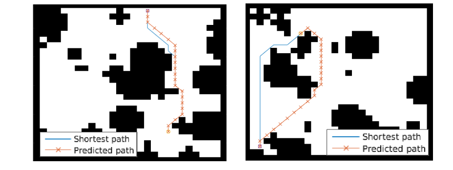
The agent gets a reward +1 in the goal state, -1 in obstacles (black), and -0.01 for each step (so that the shortest path to the goal is an optimal solution).
## VIN model
The agent is implemented in a very straight-forward manner as a single neural network trained with TRPO (Policy Gradients with a KL constraint on predictive action distributions over a batch of trajectories). So the only loss function used is to maximize expected reward, as is standard in model-free RL. However, the policy network of the agent has a very specific structure since it (internally) runs value iteration.
First, there's the core Value Iteration **(VI) Module** which runs the recurrence formula (reproducing again):

The input to this recurrence are the two arrays R (the reward array, reward for each state) and P (the dynamics array, the probabilities of transitioning to nearby states with each action), which are of course unknown to the agent, but can be predicted with neural networks as a function of the current state. This is a little funny because the networks take a _particular_ state **s** and are internally (during the forward pass) predicting the rewards and dynamics for all states and actions in the entire environment. Notice, extremely importantly and once again, that at no point are the reward and dynamics functions explicitly regressed to the observed transitions in the environment. They are just arrays of numbers that plug into value iteration recurrence module.
But anyway, once we have **R,P** arrays, in the Grid-world above due to the local connectivity, value iteration can be implemented with a repeated application of convolving **P** over **R**, as these filters effectively *diffuse* the estimated reward function (**R**) through the dynamics model (**P**), followed by max pooling across the actions. If **P** is a not a function of the state, it would simply be the filters in the Conv layer. Notice that posing this as convolution also assumes that the env dynamics are position-invariant. See the diagram below on the right: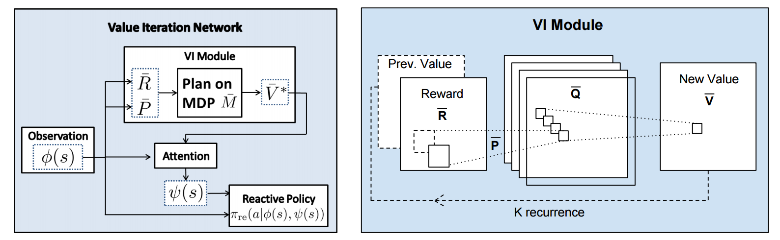
Once the array of numbers that we interpret as holding the estimated $V^*$ is computed after running **K** steps of the recurrence (K is fixed beforehand. For example for a 16x16 map it is 20, since that's a bit more than the amount of steps needed to diffuse rewards across the entire map), we "pluck out" the state-action values $Q(s,.)$ at the state the agent happens to currently be in (by an "attention" operator $\psi$), and (optionally) append these Q values to the feedforward representation of the current state $\phi(s)$, and finally predicting the action distribution.
## Experiments
**Baseline 1**: A vanilla ConvNet policy trained with TRPO. [(50 3x3 filters)\*2, 2x2 max pool, (100 3x3 filters)\*3, 2x2 max pool, FC(100), FC(4), Softmax].
**Baseline 2**: A fully convolutional network (FCN), 3 layers (with a filter that spans the whole image), of 150, 100, 10 filters. i.e. slightly different and perhaps a bit more domain-appropriate ConvNet architecture.
**Curriculum** is used during training where easier environments are trained on first. This is claimed to work better but not quantified in tables. Models are trained with TRPO, RMSProp, implemented in Theano.
Results when training on **5000** random grid-world instances (hey isn't that quite a bit low?):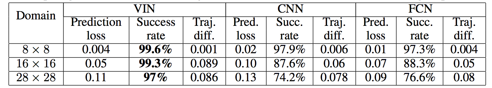
TLDR VIN generalizes better.
The authors also run the model on the **Mars Rover Navigation** dataset (wait what?), a **Continuous Control** 2D path planning dataset, and the **WebNav Challenge**, a language-based search task on a graph (of a subset of Wikipedia). Skipping these because they don't add _too_ much to the core cool idea of the paper.
## Misc
**The good**: I really like this paper because the core idea is cute (the planner is *embedded* in the policy and trained end-to-end), novel (I don't think I saw this idea executed on so far elsewhere), the paper is well-written and clear, and the supplementary materials are thorough.
**On the approach**: Significant challenges remain to make this approach more practicaly viable, but it also seems that much more exciting followup work can be done in this framework. I wish the authors discussed this more in the conclusion. In particular, it seems that one has to explicitly encode the environment connectivity structure in the internal model $\bar{M}$. How much of a problem is this and what could be done about it? Or how could we do the planning in more higher-level abstract spaces instead of the actual low-level state space of the problem? Also, it seems that a potentially nice feature of this approach is that the agent could dynamically "decide" on a reward function at runtime, and the VI module can diffuse it through the dynamics and hence do the planning. A potentially interesting outcome is that the agent could utilize this kind of computation so that an LSTM controller could learn to "emit" reward function subgoals and the VI planner computes how to meet them. A nice/clean division of labor one could hope for in principle.
**The experiments**. Unfortunately, I'm not sure why the authors preferred breadth of experiments and sacrificed depth of experiments. I would have much preferred a more in-depth analysis of the gridworld environment. For instance:
- Only 5,000 training examples are used for training, which seems very little. Presumable, the baselines get stronger as you increase the number of training examples?
- Lack of visualizations: Does the model actually learn the "correct" rewards **R** and dynamics **P**? The authors could inspect these manually and correlate them to the actual model. This would have been reaaaallllyy cool. I also wouldn't expect the model to exactly learn these, but who knows.
- How does the model compare to the baselines in the number of parameters? or FLOPS? It seems that doing VI for 30 steps at each single iteration of the algorithm should be quite expensive.
- The authors should study the performance as a function of the number of recurrences **K**. A particularly funny experiment would be K = 1, where the model would be effectively predicting **V*** directly, without planning. What happens?
- If the output of VI $\psi(s)$ is concatenated to the state parameters, are these Q values actually used? What if all the weights to these numbers are zero in the trained models?
- Why do the authors only evaluate success rate when the training criterion is expected reward?
Overall a very cute idea, well executed as a first step and well explained, with a bit of unsatisfying lack of depth in the experiments in favor of breadth that doesn't add all that much.
2 Comments
  |

Exploring the Hyperparameter Landscape of Adversarial Robustness
Duesterwald, Evelyn and Murthi, Anupama and Venkataraman, Ganesh and Sinn, Mathieu and Vijaykeerthy, Deepak
- 2019 via Local Bibsonomy
Keywords: adversarial, robustness
Duesterwald, Evelyn and Murthi, Anupama and Venkataraman, Ganesh and Sinn, Mathieu and Vijaykeerthy, Deepak
- 2019 via Local Bibsonomy
Keywords: adversarial, robustness
|
[link]
Duesterwald et al. study the influence of hyperparameters on adversarial training and its robustness as well as accuracy. As shown in Figure 1, the chosen parameters, the ratio of adversarial examples per batch and the allowed perturbation $\epsilon$, allow to control the trade-off between adversarial robustness and accuracy. Even for larger $\epsilon$, at least on MNIST and SVHN, using only few adversarial examples per batch increases robustness significantly while only incurring a small loss in accuracy. https://i.imgur.com/nMZNpFB.jpg Figure 1: Robustness (red) and accuracy (blue) depending on the two hyperparameters $\epsilon$ and ratio of adversarial examples per batch. Robustness is measured in adversarial accuracy. Also find this summary at [davidstutz.de](https://davidstutz.de/category/reading/). |
