
|
Welcome to ShortScience.org! |


|
- ShortScience.org is a platform for post-publication discussion aiming to improve accessibility and reproducibility of research ideas.
- The website has 1584 public summaries, mostly in machine learning, written by the community and organized by paper, conference, and year.
- Reading summaries of papers is useful to obtain the perspective and insight of another reader, why they liked or disliked it, and their attempt to demystify complicated sections.
- Also, writing summaries is a good exercise to understand the content of a paper because you are forced to challenge your assumptions when explaining it.
- Finally, you can keep up to date with the flood of research by reading the latest summaries on our Twitter and Facebook pages.
Generating Images with Perceptual Similarity Metrics based on Deep Networks
Alexey Dosovitskiy and Thomas Brox
arXiv e-Print archive - 2016 via Local arXiv
Keywords: cs.LG, cs.CV, cs.NE
First published: 2016/02/08 (8 years ago)
Abstract: Image-generating machine learning models are typically trained with loss functions based on distance in the image space. This often leads to over-smoothed results. We propose a class of loss functions, which we call deep perceptual similarity metrics (DeePSiM), that mitigate this problem. Instead of computing distances in the image space, we compute distances between image features extracted by deep neural networks. This metric better reflects perceptually similarity of images and thus leads to better results. We show three applications: autoencoder training, a modification of a variational autoencoder, and inversion of deep convolutional networks. In all cases, the generated images look sharp and resemble natural images.
more
less
Alexey Dosovitskiy and Thomas Brox
arXiv e-Print archive - 2016 via Local arXiv
Keywords: cs.LG, cs.CV, cs.NE
First published: 2016/02/08 (8 years ago)
Abstract: Image-generating machine learning models are typically trained with loss functions based on distance in the image space. This often leads to over-smoothed results. We propose a class of loss functions, which we call deep perceptual similarity metrics (DeePSiM), that mitigate this problem. Instead of computing distances in the image space, we compute distances between image features extracted by deep neural networks. This metric better reflects perceptually similarity of images and thus leads to better results. We show three applications: autoencoder training, a modification of a variational autoencoder, and inversion of deep convolutional networks. In all cases, the generated images look sharp and resemble natural images.


[link]
* The authors define in this paper a special loss function (DeePSiM), mostly for autoencoders.
* Usually one would use a MSE of euclidean distance as the loss function for an autoencoder. But that loss function basically always leads to blurry reconstructed images.
* They add two new ingredients to the loss function, which results in significantly sharper looking images.
### How
* Their loss function has three components:
* Euclidean distance in image space (i.e. pixel distance between reconstructed image and original image, as usually used in autoencoders)
* Euclidean distance in feature space. Another pretrained neural net (e.g. VGG, AlexNet, ...) is used to extract features from the original and the reconstructed image. Then the euclidean distance between both vectors is measured.
* Adversarial loss, as usually used in GANs (generative adversarial networks). The autoencoder is here treated as the GAN-Generator. Then a second network, the GAN-Discriminator is introduced. They are trained in the typical GAN-fashion. The loss component for DeePSiM is the loss of the Discriminator. I.e. when reconstructing an image, the autoencoder would learn to reconstruct it in a way that lets the Discriminator believe that the image is real.
* Using the loss in feature space alone would not be enough as that tends to lead to overpronounced high frequency components in the image (i.e. too strong edges, corners, other artefacts).
* To decrease these high frequency components, a "natural image prior" is usually used. Other papers define some function by hand. This paper uses the adversarial loss for that (i.e. learns a good prior).
* Instead of training a full autoencoder (encoder + decoder) it is also possible to only train a decoder and feed features - e.g. extracted via AlexNet - into the decoder.
### Results
* Using the DeePSiM loss with a normal autoencoder results in sharp reconstructed images.
* Using the DeePSiM loss with a VAE to generate ILSVRC-2012 images results in sharp images, which are locally sound, but globally don't make sense. Simple euclidean distance loss results in blurry images.
* Using the DeePSiM loss when feeding only image space features (extracted via AlexNet) into the decoder leads to high quality reconstructions. Features from early layers will lead to more exact reconstructions.
* One can again feed extracted features into the network, but then take the reconstructed image, extract features of that image and feed them back into the network. When using DeePSiM, even after several iterations of that process the images still remain semantically similar, while their exact appearance changes (e.g. a dog's fur color might change, counts of visible objects change).
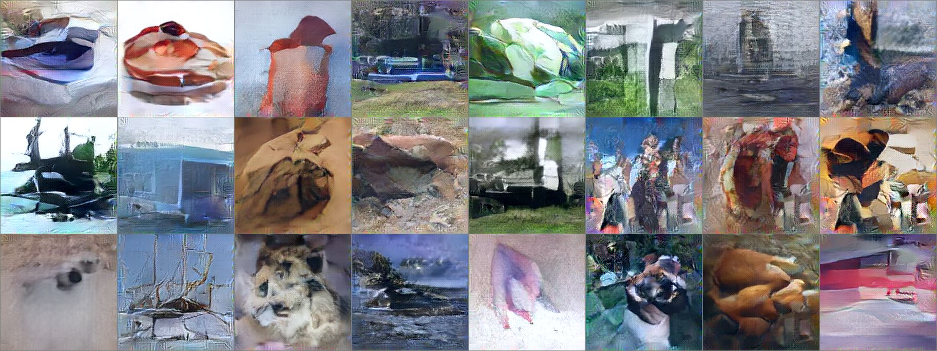
*Images generated with a VAE using DeePSiM loss.*
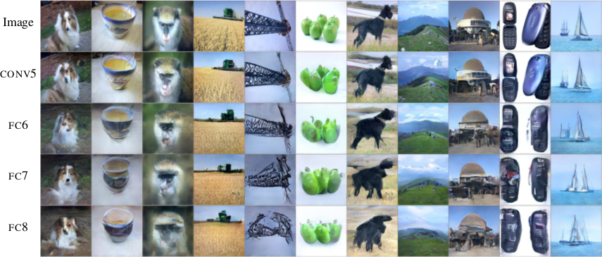
*Images reconstructed from features fed into the network. Different AlexNet layers (conv5 - fc8) were used to generate the features. Earlier layers allow more exact reconstruction.*
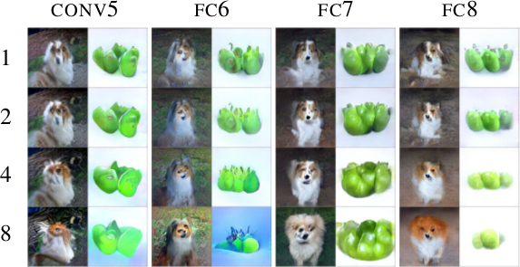
*First, images are reconstructed from features (AlexNet, layers conv5 - fc8 as columns). Then, features of the reconstructed images are fed back into the network. That is repeated up to 8 times (rows). Images stay semantically similar, but their appearance changes.*
--------------------
### Rough chapter-wise notes
* (1) Introduction
* Using a MSE of euclidean distances for image generation (e.g. autoencoders) often results in blurry images.
* They suggest a better loss function that cares about the existence of features, but not as much about their exact translation, rotation or other local statistics.
* Their loss function is based on distances in suitable feature spaces.
* They use ConvNets to generate those feature spaces, as these networks are sensitive towards important changes (e.g. edges) and insensitive towards unimportant changes (e.g. translation).
* However, naively using the ConvNet features does not yield good results, because the networks tend to project very different images onto the same feature vectors (i.e. they are contractive). That leads to artefacts in the generated images.
* Instead, they combine the feature based loss with GANs (adversarial loss). The adversarial loss decreases the negative effects of the feature loss ("natural image prior").
* (3) Model
* A typical choice for the loss function in image generation tasks (e.g. when using an autoencoders) would be squared euclidean/L2 loss or L1 loss.
* They suggest a new class of losses called "DeePSiM".
* We have a Generator `G`, a Discriminator `D`, a feature space creator `C` (takes an image, outputs a feature space for that image), one (or more) input images `x` and one (or more) target images `y`. Input and target image can be identical.
* The total DeePSiM loss is a weighted sum of three components:
* Feature loss: Squared euclidean distance between the feature spaces of (1) input after fed through G and (2) the target image, i.e. `||C(G(x))-C(y)||^2_2`.
* Adversarial loss: A discriminator is introduced to estimate the "fakeness" of images generated by the generator. The losses for D and G are the standard GAN losses.
* Pixel space loss: Classic squared euclidean distance (as commonly used in autoencoders). They found that this loss stabilized their adversarial training.
* The feature loss alone would create high frequency artefacts in the generated image, which is why a second loss ("natural image prior") is needed. The adversarial loss fulfills that role.
* Architectures
* Generator (G):
* They define different ones based on the task.
* They all use up-convolutions, which they implement by stacking two layers: (1) a linear upsampling layer, then (2) a normal convolutional layer.
* They use leaky ReLUs (alpha=0.3).
* Comparators (C):
* They use variations of AlexNet and Exemplar-CNN.
* They extract the features from different layers, depending on the experiment.
* Discriminator (D):
* 5 convolutions (with some striding; 7x7 then 5x5, afterwards 3x3), into average pooling, then dropout, then 2x linear, then 2-way softmax.
* Training details
* They use Adam with learning rate 0.0002 and normal momentums (0.9 and 0.999).
* They temporarily stop the discriminator training when it gets too good.
* Batch size was 64.
* 500k to 1000k batches per training.
* (4) Experiments
* Autoencoder
* Simple autoencoder with an 8x8x8 code layer between encoder and decoder (so actually more values than in the input image?!).
* Encoder has a few convolutions, decoder a few up-convolutions (linear upsampling + convolution).
* They train on STL-10 (96x96) and take random 64x64 crops.
* Using for C AlexNet tends to break small structural details, using Exempler-CNN breaks color details.
* The autoencoder with their loss tends to produce less blurry images than the common L2 and L1 based losses.
* Training an SVM on the 8x8x8 hidden layer performs significantly with their loss than L2/L1. That indicates potential for unsupervised learning.
* Variational Autoencoder
* They replace part of the standard VAE loss with their DeePSiM loss (keeping the KL divergence term).
* Everything else is just like in a standard VAE.
* Samples generated by a VAE with normal loss function look very blurry. Samples generated with their loss function look crisp and have locally sound statistics, but still (globally) don't really make any sense.
* Inverting AlexNet
* Assume the following variables:
* I: An image
* ConvNet: A convolutional network
* F: The features extracted by a ConvNet, i.e. ConvNet(I) (feaures in all layers, not just the last one)
* Then you can invert the representation of a network in two ways:
* (1) An inversion that takes an F and returns roughly the I that resulted in F (it's *not* key here that ConvNet(reconstructed I) returns the same F again).
* (2) An inversion that takes an F and projects it to *some* I so that ConvNet(I) returns roughly the same F again.
* Similar to the autoencoder cases, they define a decoder, but not encoder.
* They feed into the decoder a feature representation of an image. The features are extracted using AlexNet (they try the features from different layers).
* The decoder has to reconstruct the original image (i.e. inversion scenario 1). They use their DeePSiM loss during the training.
* The images can be reonstructed quite well from the last convolutional layer in AlexNet. Chosing the later fully connected layers results in more errors (specifially in the case of the very last layer).
* They also try their luck with the inversion scenario (2), but didn't succeed (as their loss function does not care about diversity).
* They iteratively encode and decode the same image multiple times (probably means: image -> features via AlexNet -> decode -> reconstructed image -> features via AlexNet -> decode -> ...). They observe, that the image does not get "destroyed", but rather changes semantically, e.g. three apples might turn to one after several steps.
* They interpolate between images. The interpolations are smooth.
 |

Group Normalization
Yuxin Wu and Kaiming He
arXiv e-Print archive - 2018 via Local arXiv
Keywords: cs.CV, cs.LG
First published: 2018/03/22 (6 years ago)
Abstract: Batch Normalization (BN) is a milestone technique in the development of deep learning, enabling various networks to train. However, normalizing along the batch dimension introduces problems --- BN's error increases rapidly when the batch size becomes smaller, caused by inaccurate batch statistics estimation. This limits BN's usage for training larger models and transferring features to computer vision tasks including detection, segmentation, and video, which require small batches constrained by memory consumption. In this paper, we present Group Normalization (GN) as a simple alternative to BN. GN divides the channels into groups and computes within each group the mean and variance for normalization. GN's computation is independent of batch sizes, and its accuracy is stable in a wide range of batch sizes. On ResNet-50 trained in ImageNet, GN has 10.6% lower error than its BN counterpart when using a batch size of 2; when using typical batch sizes, GN is comparably good with BN and outperforms other normalization variants. Moreover, GN can be naturally transferred from pre-training to fine-tuning. GN can outperform its BN-based counterparts for object detection and segmentation in COCO, and for video classification in Kinetics, showing that GN can effectively replace the powerful BN in a variety of tasks. GN can be easily implemented by a few lines of code in modern libraries.
more
less
Yuxin Wu and Kaiming He
arXiv e-Print archive - 2018 via Local arXiv
Keywords: cs.CV, cs.LG
First published: 2018/03/22 (6 years ago)
Abstract: Batch Normalization (BN) is a milestone technique in the development of deep learning, enabling various networks to train. However, normalizing along the batch dimension introduces problems --- BN's error increases rapidly when the batch size becomes smaller, caused by inaccurate batch statistics estimation. This limits BN's usage for training larger models and transferring features to computer vision tasks including detection, segmentation, and video, which require small batches constrained by memory consumption. In this paper, we present Group Normalization (GN) as a simple alternative to BN. GN divides the channels into groups and computes within each group the mean and variance for normalization. GN's computation is independent of batch sizes, and its accuracy is stable in a wide range of batch sizes. On ResNet-50 trained in ImageNet, GN has 10.6% lower error than its BN counterpart when using a batch size of 2; when using typical batch sizes, GN is comparably good with BN and outperforms other normalization variants. Moreover, GN can be naturally transferred from pre-training to fine-tuning. GN can outperform its BN-based counterparts for object detection and segmentation in COCO, and for video classification in Kinetics, showing that GN can effectively replace the powerful BN in a variety of tasks. GN can be easily implemented by a few lines of code in modern libraries.
|
[link]
If you were to survey researchers, and ask them to name the 5 most broadly influential ideas in Machine Learning from the last 5 years, I’d bet good money that Batch Normalization would be somewhere on everyone’s lists. Before Batch Norm, training meaningfully deep neural networks was an unstable process, and one that often took a long time to converge to success. When we added Batch Norm to models, it allowed us to increase our learning rates substantially (leading to quicker training) without the risk of activations either collapsing or blowing up in values. It had this effect because it addressed one of the key difficulties of deep networks: internal covariate shift. To understand this, imagine the smaller problem, of a one-layer model that’s trying to classify based on a set of input features. Now, imagine that, over the course of training, the input distribution of features moved around, so that, perhaps, a value that was at the 70th percentile of the data distribution initially is now at the 30th. We have an obvious intuition that this would make the model quite hard to train, because it would learn some mapping between feature values and class at the beginning of training, but that would become invalid by the end. This is, fundamentally, the problem faced by higher layers of deep networks, since, if the distribution of activations in a lower layer changed even by a small amount, that can cause a “butterfly effect” style outcome, where the activation distributions of higher layers change more dramatically. Batch Normalization - which takes each feature “channel” a network learns, and normalizes [normalize = subtract mean, divide by variance] it by the mean and variance of that feature over spatial locations and over all the observations in a given batch - helps solve this problem because it ensures that, throughout the course of training, the distribution of inputs that a given layer sees stays roughly constant, no matter what the lower layers get up to. On the whole, Batch Norm has been wildly successful at stabilizing training, and is now canonized - along with the likes of ReLU and Dropout - as one of the default sensible training procedures for any given network. However, it does have its difficulties and downsides. One salient one of these comes about when you train using very small batch sizes - in the range of 2-16 examples per batch. Under these circumstance, the mean and variance calculated off of that batch are noisy and high variance (for the general reason that statistics calculated off of small sample sizes are noisy and high variance), which takes away from the stability that Batch Norm is trying to provide. One proposed alternative to Batch Norm, that didn’t run into this problem of small sample sizes, is Layer Normalization. This operates under the assumption that the activations of all feature “channels” within a given layer hopefully have roughly similar distributions, and, so, you an normalize all of them by taking the aggregate mean over all channels, *for a given observation*, and use that as the mean and variance you normalize by. Because there are typically many channels in a given layer, this means that you have many “samples” that go into the mean and variance. However, this assumption - that the distributions for each feature channel are roughly the same - can be an incorrect one. A useful model I have for thinking about the distinction between these two approaches is the idea that both are calculating approximations of an underlying abstract notion: the in-the-limit mean and variance of a single feature channel, at a given point in time. Batch Normalization is an approximation of that insofar as it only has a small sample of points to work with, and so its estimate will tend to be high variance. Layer Normalization is an approximation insofar as it makes the assumption that feature distributions are aligned across channels: if this turns out not to be the case, individual channels will have normalizations that are biased, due to being pulled towards the mean and variance calculated over an aggregate of channels that are different than them. Group Norm tries to find a balance point between these two approaches, one that uses multiple channels, and normalizes within a given instance (to avoid the problems of small batch size), but, instead of calculating the mean and variance over all channels, calculates them over a group of channels that represents a subset. The inspiration for this idea comes from the fact that, in old school computer vision, it was typical to have parts of your feature vector that - for example - represented a histogram of some value (say: localized contrast) over the image. Since these multiple values all corresponded to a larger shared “group” feature. If a group of features all represent a similar idea, then their distributions will be more likely to be aligned, and therefore you have less of the bias issue. One confusing element of this paper for me was that the motivation part of the paper strongly implied that the reason group norm is sensible is that you are able to combine statistically dependent channels into a group together. However, as far as I an tell, there’s no actually clustering or similarity analysis of channels that is done to place certain channels into certain groups; it’s just done so semi-randomly based on the index location within the feature channel vector. So, under this implementation, it seems like the benefits of group norm are less because of any explicit seeking out of dependant channels, and more that just having fewer channels in each group means that each individual channel makes up more of the weight in its group, which does something to reduce the bias effect anyway. The upshot of the Group Norm paper, results-wise, is that Group Norm performs better than both Batch Norm and Layer Norm at very low batch sizes. This is useful if you’re training on very dense data (e.g. high res video), where it might be difficult to store more than a few observations in memory at a time. However, once you get to batch sizes of ~24, Batch Norm starts to do better, presumably since that’s a large enough sample size to reduce variance, and you get to the point where the variance of BN is preferable to the bias of GN. |

Mask R-CNN
He, Kaiming and Gkioxari, Georgia and Dollár, Piotr and Girshick, Ross B.
arXiv e-Print archive - 2017 via Local Bibsonomy
Keywords: dblp
He, Kaiming and Gkioxari, Georgia and Dollár, Piotr and Girshick, Ross B.
arXiv e-Print archive - 2017 via Local Bibsonomy
Keywords: dblp
|
[link]
Mask RCNN takes off from where Faster RCNN left, with some augmentations aimed at bettering instance segmentation (which was out of scope for FRCNN). Instance segmentation was achieved remarkably well in *DeepMask* , *SharpMask* and later *Feature Pyramid Networks* (FPN). Faster RCNN was not designed for pixel-to-pixel alignment between network inputs and outputs. This is most evident in how RoIPool , the de facto core operation for attending to instances, performs coarse spatial quantization for feature extraction. Mask RCNN fixes that by introducing RoIAlign in place of RoIPool. #### Methodology Mask RCNN retains most of the architecture of Faster RCNN. It adds the a third branch for segmentation. The third branch takes the output from RoIAlign layer and predicts binary class masks for each class. ##### Major Changes and intutions **Mask prediction** Mask prediction segmentation predicts a binary mask for each RoI using fully convolution - and the stark difference being usage of *sigmoid* activation for predicting final mask instead of *softmax*, implies masks don't compete with each other. This *decouples* segmentation from classification. The class prediction branch is used for class prediction and for calculating loss, the mask of predicted loss is used calculating Lmask. Also, they show that a single class agnostic mask prediction works almost as effective as separate mask for each class, thereby supporting their method of decoupling classification from segmentation **RoIAlign** RoIPool first quantizes a floating-number RoI to the discrete granularity of the feature map, this quantized RoI is then subdivided into spatial bins which are themselves quantized, and finally feature values covered by each bin are aggregated (usually by max pooling). Instead of quantization of the RoI boundaries or bin bilinear interpolation is used to compute the exact values of the input features at four regularly sampled locations in each RoI bin, and aggregate the result (using max or average). **Backbone architecture** Faster RCNN uses a VGG like structure for extracting features from image, weights of which were shared among RPN and region detection layers. Herein, authors experiment with 2 backbone architectures - ResNet based VGG like in FRCNN and ResNet based [FPN](http://www.shortscience.org/paper?bibtexKey=journals/corr/LinDGHHB16) based. FPN uses convolution feature maps from previous layers and recombining them to produce pyramid of feature maps to be used for prediction instead of single-scale feature layer (final output of conv layer before connecting to fc layers was used in Faster RCNN) **Training Objective** The training objective looks like this  Lmask is the addition from Faster RCNN. The method to calculate was mentioned above #### Observation Mask RCNN performs significantly better than COCO instance segmentation winners *without any bells and whiskers*. Detailed results are available in the paper |

Rich Feature Hierarchies for Accurate Object Detection and Semantic Segmentation
Girshick, Ross B. and Donahue, Jeff and Darrell, Trevor and Malik, Jitendra
Conference and Computer Vision and Pattern Recognition - 2014 via Local Bibsonomy
Keywords: dblp
Girshick, Ross B. and Donahue, Jeff and Darrell, Trevor and Malik, Jitendra
Conference and Computer Vision and Pattern Recognition - 2014 via Local Bibsonomy
Keywords: dblp
|
[link]
# Object detection system overview.

https://i.imgur.com/vd2YUy3.png

1.	takes an input image,
2.	extracts around 2000 bottom-up region proposals,
3.	computes features for each proposal using a large convolutional neural network (CNN), and then
4.	classifies each region using class-specific linear SVMs.
* R-CNN achieves a mean average precision (mAP) of 53.7% on PASCAL VOC 2010.
* On the 200-class ILSVRC2013 detection dataset, R-CNN’s mAP is 31.4%, a large improvement over OverFeat , which had the previous best result at 24.3%.

## There is a 2 challenges faced in object detection
1.	localization problem
2.	labeling the data

1 localization problem :
*  One approach frames localization as a regression problem.  they report a mAP of 30.5% on VOC 2007 compared to the 58.5% achieved by our method.
* An alternative is to build a sliding-window detector.  considered adopting a sliding-window approach increases the number of convolutional layers to 5, have very large receptive fields (195 x 195 pixels) and strides (32x32 pixels) in the input image, which makes precise localization within the sliding-window paradigm.

2 labeling the data:
* The conventional solution to this problem is to use unsupervised pre-training, followed by supervise fine-tuning
* supervised pre-training on a large auxiliary dataset (ILSVRC), followed by domain specific fine-tuning on a small dataset (PASCAL),
* fine-tuning for detection improves mAP performance by 8 percentage points.
* Stochastic gradient descent via back propagation was used to  effective for training convolutional neural networks (CNNs)

##  Object detection with R-CNN
This  system consists of three modules
* The first generates category-independent region proposals. These proposals define the set of candidate detections available to our detector.
*  The second module is a large convolutional neural network that extracts a fixed-length feature vector from each region.
* The third module is a set of class specific linear SVMs.

Module design

1 Region proposals
* which detect mitotic cells by applying a CNN to regularly-spaced square crops.
* use selective search method in fast mode (Capture All Scales, Diversification, Fast to Compute).
* the time spent computing region proposals and features (13s/image on a GPU or 53s/image on a CPU)

2 Feature extraction.
* extract a 4096-dimensional feature vector from each region proposal using the Caffe  implementation of the CNN
* Features are computed by forward propagating a mean-subtracted 227x227 RGB image through five convolutional layers and two fully connected layers.
* warp all pixels in a tight bounding box around it to the required size
* The feature matrix is typically 2000x4096

3 Test time detection
* At test time, run selective search on the test image to extract around 2000 region proposals (we use selective search’s “fast mode” in all experiments).
*  warp each proposal and forward propagate it through the CNN in order to compute features. Then, for each class, we score each extracted feature vector using the SVM trained for that class.
* Given all scored regions in an image, we apply a greedy non-maximum suppression (for each class independently) that rejects a region if it has an intersection-over union (IoU) overlap with a higher scoring selected region larger than a learned threshold.
## Training

1 Supervised pre-training:
 * pre-trained the CNN on a large auxiliary dataset (ILSVRC2012 classification)  using image-level annotations only (bounding box labels are not available for this data)

2  Domain-specific fine-tuning.
* use the stochastic gradient descent (SGD) training of the CNN parameters using only warped region proposals with  learning rate of 0.001.

3  Object category classifiers.
*   use intersection-over union (IoU) overlap threshold method  to label a region with The overlap threshold of 0.3.
* Once features are extracted and training labels are applied, we optimize one linear SVM per class.
* adopt the standard hard negative mining method to fit large training data in memory.

### Results on PASCAL VOC 201012

1  VOC 2010
* compared against four strong baselines including SegDPM, DPM, UVA, Regionlets.
* Achieve a large improvement in mAP, from 35.1% to 53.7% mAP,  while also being much faster
 https://i.imgur.com/0dGX9b7.png
2 ILSVRC2013 detection.
* ran R-CNN on the 200-class ILSVRC2013 detection dataset
* R-CNN achieves a mAP of 31.4%
https://i.imgur.com/GFbULx3.png
#### Performance layer-by-layer, without fine-tuning
1 pool5 layer
* which is the max pooled output of the network’s fifth and final convolutional layer.
*The pool5 feature map is 6 x6 x 256 = 9216 dimensional
* each pool5 unit has a receptive field of 195x195 pixels in the original 227x227 pixel input

2 Layer fc6
* fully connected to pool5
*  it multiplies a 4096x9216 weight matrix by the pool5 feature map (reshaped as a 9216-dimensional vector) and then adds a vector of biases

3 Layer fc7
* It is implemented by multiplying the features computed by fc6 by a 4096 x 4096 weight matrix, and similarly adding a vector of biases and applying half-wave rectification
#### Performance layer-by-layer, with fine-tuning
* CNN’s parameters  fine-tuned on PASCAL.
* fine-tuning increases mAP by 8.0 % points to 54.2%

### Network architectures
* 16-layer deep network, consisting of 13 layers of 3 _ 3 convolution kernels, with five max pooling layers interspersed, and topped with three fully-connected layers. We refer to this network as “O-Net” for OxfordNet and the baseline as “T-Net” for TorontoNet.
* RCNN with O-Net substantially outperforms R-CNN with TNet, increasing mAP from 58.5% to 66.0%
* drawback in terms of compute time, with in terms of compute time, with than T-Net.

1 The ILSVRC2013 detection dataset
* dataset is split into three sets: train (395,918), val (20,121), and test (40,152)

#### CNN features for segmentation.
* full R-CNN: The first strategy (full) ignores the re region’s shape and computes CNN features directly on the warped window. Two regions might have very similar bounding boxes while having very little overlap.
* fg R-CNN: the second strategy (fg) computes CNN features only on a region’s foreground mask. We replace the background with the mean input so that background regions are zero after mean subtraction.
* full+fg R-CNN: The third strategy (full+fg) simply concatenates the full and fg features
 https://i.imgur.com/n1bhmKo.png
1 Comments
 |

Reward Augmented Maximum Likelihood for Neural Structured Prediction
Mohammad Norouzi and Samy Bengio and Zhifeng Chen and Navdeep Jaitly and Mike Schuster and Yonghui Wu and Dale Schuurmans
arXiv e-Print archive - 2016 via Local arXiv
Keywords: cs.LG
First published: 2016/09/01 (7 years ago)
Abstract: A key problem in structured output prediction is direct optimization of the task reward function that matters for test evaluation. This paper presents a simple and computationally efficient approach to incorporate task reward into a maximum likelihood framework. We establish a connection between the log-likelihood and regularized expected reward objectives, showing that at a zero temperature, they are approximately equivalent in the vicinity of the optimal solution. We show that optimal regularized expected reward is achieved when the conditional distribution of the outputs given the inputs is proportional to their exponentiated (temperature adjusted) rewards. Based on this observation, we optimize conditional log-probability of edited outputs that are sampled proportionally to their scaled exponentiated reward. We apply this framework to optimize edit distance in the output label space. Experiments on speech recognition and machine translation for neural sequence to sequence models show notable improvements over a maximum likelihood baseline by using edit distance augmented maximum likelihood.
more
less
Mohammad Norouzi and Samy Bengio and Zhifeng Chen and Navdeep Jaitly and Mike Schuster and Yonghui Wu and Dale Schuurmans
arXiv e-Print archive - 2016 via Local arXiv
Keywords: cs.LG
First published: 2016/09/01 (7 years ago)
Abstract: A key problem in structured output prediction is direct optimization of the task reward function that matters for test evaluation. This paper presents a simple and computationally efficient approach to incorporate task reward into a maximum likelihood framework. We establish a connection between the log-likelihood and regularized expected reward objectives, showing that at a zero temperature, they are approximately equivalent in the vicinity of the optimal solution. We show that optimal regularized expected reward is achieved when the conditional distribution of the outputs given the inputs is proportional to their exponentiated (temperature adjusted) rewards. Based on this observation, we optimize conditional log-probability of edited outputs that are sampled proportionally to their scaled exponentiated reward. We apply this framework to optimize edit distance in the output label space. Experiments on speech recognition and machine translation for neural sequence to sequence models show notable improvements over a maximum likelihood baseline by using edit distance augmented maximum likelihood.
|
[link]
(See also a more thorough summary in [a LaTeX PDF][1].)

This paper has some nice clear theory which bridges maximum likelihood (supervised) learning and standard reinforcement learning. It focuses on *structured prediction* tasks, where we want to learn to predict $p_\theta(y \mid x)$ where $y$ is some object with complex internal structure.

We can agree on some deficiencies of maximum likelihood learning:

- ML training fails to assign **partial credit**. Models are trained to maximize the likelihood of the ground-truth outputs in the dataset, and all other outputs are equally wrong. This is an increasingly important problem as the space of possible solutions grows.
- ML training is potentially disconnected from **downstream task reward**. In machine translation, we usually want to optimize relatively complex metrics like BLEU or TER. Since these metrics are non-differentiable, we have to settle for optimizing proxy losses that we hope are related to the metric of interest.

Reinforcement learning offers an attractive alternative in theory. RL algorithms are designed to optimize non-differentiable (even stochastic) reward functions, which sounds like just what we want. But RL algorithms have their own problems with this sort of structured output space:

- Standard RL algorithms rely on samples from the model we are learning, $p_\theta(y \mid x)$. This becomes intractable when our output space is very complex (e.g. 80-token sequences where each word is drawn from a vocabulary of 80,000 words).
- The reward spaces for problems of interest are extremely sparse. Our metrics will assign 0 reward to most of the 80^80K possible outputs in the translation problem in the paper.
- Vanilla RL doesn't take into account the ground-truth outputs available to us in structured prediction.

This paper designs a solution which combines supervised learning with a reinforcement learning-inspired smoothing method. Concretely, the authors design an **exponentiated payoff distribution** $q(y \mid y^*; \tau)$ which assigns high mass to high-reward outputs $y$ and low mass elsewhere. This distribution is used to effectively smooth the loss function established by the ground-truth outputs in the supervised data. We end up optimizing the following objective:

$$\mathcal L_\text{RML} = - \mathbb E_{x, y^* \sim \mathcal D}\left[ \sum_y q(y \mid y^*; \tau) \log p_\theta(y \mid x) \right]$$

This optimization depends on samples from our dataset $\mathcal D$ and, more importantly, the stationary payoff distribution $q$. This contrasts strongly with standard RL training, where the objective depends on samples from the non-stationary model distribution $p_\theta$. To make that clear, we can rewrite the above with another expectation:

$$\mathcal L_\text{RML} = - \mathbb E_{x, y^* \sim \mathcal D, y \sim q(y \mid y^*; \tau)}\left[ \log p_\theta(y \mid x) \right]$$

### Model details

If you're interested in the low-level details, I wrote up the gist of the math in [this PDF][1].

### Analysis

#### Relationship to label smoothing

This training approach is mathematically equivalent to label smoothing, applied here to structured output problems. In next-word prediction language modeling, a popular trick involves smoothing the target distributions by combining the ground-truth output with some simple base model, e.g. a unigram word frequency distribution. (This just means we take a weighted sum of the one-hot vector from our supervised data and a normalized frequency vector calculated on some corpus.) Mathematically, the cross entropy with label smoothing is

$$\mathcal L_\text{ML-smooth} = - \mathbb E_{x, y^* \sim \mathcal D} \left[ \sum_y p_\text{smooth}(y; y^*) \log p_\theta(y \mid x) \right]$$

(The equation above leaves out a constant entropy term.)

The gradient of this objective looks exactly the same as the reward-augmented ML gradient from the paper:

$$\nabla_\theta \mathcal L_\text{ML-smooth} = \mathbb E_{x, y^* \sim \mathcal D, y \sim p_\text{smooth}} \left[ \log p_\theta(y \mid x) \right]$$

So reward-augmented likelihood is equivalent to label smoothing, where our smoothing distribution is log-proportional to our downstream reward function.

#### Relationship to distillation

Optimizing the reward-augmented maximum likelihood is equivalent to minimizing the KL divergence $$D_\text{KL}(q(y \mid y^*; \tau) \mid\mid p_\theta(y \mid x))$$

This divergence reaches zero iff $q = p$. We can say, then, that the effect of optimizing on $\mathcal L_\text{RML}$ is to **distill** the reward function (which parameterizes $q$) into the model parameters $\theta$ (which parameterize $p_\theta$).

It's exciting to think about other sorts of more complex models that we might be able to distill in this framework. The unfortunate (?) restriction is that the "source" model of the distillation ($q$ in this paper) must admit to efficient sampling.

#### Relationship to adversarial training

We can also view reward-augmented maximum likelihood training as a data augmentation technique: it synthesizes new "partially correct" examples using the reward function as a guide. We then train on all of the original and synthesized data, again weighting the gradients based on the reward function.

Adversarial training is a similar data augmentation technique which generates examples that force the model to be robust to changes in its input space (robust to changes of $x$). Both adversarial training and the RML objective encourage the model to be robust "near" the ground-truth supervised data. A high-level comparison:

- Adversarial training can be seen as data augmentation in the input space; RML training performs data augmentation in the output space.
- Adversarial training is a **model-based data augmentation**: the samples are generated from a process that depends on the current parameters during training. RML training performs **data-based augmentation**, which could in theory be done independent of the actual training process.

---

Thanks to Andrej Karpathy, Alec Radford, and Tim Salimans for interesting discussion which contributed to this summary.

[1]: https://drive.google.com/file/d/0B3Rdm_P3VbRDVUQ4SVBRYW82dU0/view
|
