
arXiv is an e-print service in the fields of physics, mathematics, computer science, quantitative biology, quantitative finance and statistics.
- 1996 1
- 2010 1
- 2011 1
- 2012 7
- 2013 29
- 2014 40
- 2015 130
- 2016 229
- 2017 179
- 2018 138
- 2019 95
- 2020 32
- 2021 10
- 2022 7
- 2023 3
Objective-Reinforced Generative Adversarial Networks (ORGAN) for Sequence Generation Models
Guimaraes, Gabriel Lima and Sanchez-Lengeling, Benjamin and Farias, Pedro Luis Cunha and Aspuru-Guzik, Alán
arXiv e-Print archive - 2017 via Local Bibsonomy
Keywords: dblp
Guimaraes, Gabriel Lima and Sanchez-Lengeling, Benjamin and Farias, Pedro Luis Cunha and Aspuru-Guzik, Alán
arXiv e-Print archive - 2017 via Local Bibsonomy
Keywords: dblp


[link]
This paper's proposed method, the cleverly named ORGAN, combines techniques from GANs and reinforcement learning to generate candidate molecular sequences that incentivize desirable properties while still remaining plausibly on-distribution. Prior papers I've read on molecular generation have by and large used approaches based in maximum likelihood estimation (MLE) - where you construct some distribution over molecular representations, and maximize the probability of your true data under that distribution. However, MLE methods can't be less powerful when it comes to incentivizing your model to precisely conform with structural details of your target data distribution. Generative Adversarial Networks (GANs) on the other hand, use a discriminator loss that directly penalizes your generator for being recognizably different from the true data. However, GANs have historically been difficult to use on data like the string-based molecular representations used in this paper. That's because strings are made up of discrete characters, which need to be sampled from underlying distributions, and we don't naively have good ways of making sampling from discrete distributions a differentiable process. SeqGAN was proposed to remedy this: instead of using the discriminator loss directly as the generator's loss - which would require backpropogating through the sampling operation - the generator is trained with reinforcement learning, using the discriminator score as a reward function. Each addition of an element to the sequence - or, in our case, each addition of a character to our molecular representation string - represents an action, and full sequences are rewarded based on the extent to which they resemble true sequences. https://i.imgur.com/dqtcJDU.png This paper proposes taking that model as a base, but then adding a more actually-reward-oriented reward onto it, incentivizing the model to produce molecules that have certain predicted properties, as determined by a (also very not differentiable) external molecular simulator. So, just taking a weighted sum of discriminator loss and reward, and using that as your RL reward. After all, if you're already using the policy gradient structures of RL to train the underlying generator, you might as well add on some more traditional-looking RL rewards. The central intuition behind using RL in both of these cases is that it provides a way of using training signals that are unknown or - more to the point - non-differentiable functions functions of model output. In their empirical tests focusing on molecules, the authors target the RL to optimize for one of solubility, synthesizability, and druggability (three well-defined properties within molecular simulator RDKit), as well as for uniqueness, penalizing any molecule that had been generated already. https://i.imgur.com/WszVd1M.png For all that this is an interesting mechanic, the empirical results are more equivocal. Compared to Naive RL, which directly optimizes for reward without the discriminator loss, ORGAN (Or, ORWGAN, the better-performing method using a Wasserstein GAN) doesn't have notably better rates of how often its generated strings are valid, and (as you would expect) performs comparably or slightly worse when it comes to optimizing the underlying reward. It does exhibit higher diversity than naive RL on two of the three tasks, but it's hard to get an intuition for the scales involved, and how much that scale of diversity increase would impact real results.  |

Neural Message Passing for Quantum Chemistry
Gilmer, Justin and Schoenholz, Samuel S. and Riley, Patrick F. and Vinyals, Oriol and Dahl, George E.
arXiv e-Print archive - 2017 via Local Bibsonomy
Keywords: dblp
Gilmer, Justin and Schoenholz, Samuel S. and Riley, Patrick F. and Vinyals, Oriol and Dahl, George E.
arXiv e-Print archive - 2017 via Local Bibsonomy
Keywords: dblp
|
[link]
In the years before this paper came out in 2017, a number of different graph convolution architectures - which use weight-sharing and order-invariant operations to create representations at nodes in a graph that are contextualized by information in the rest of the graph - had been suggested for learning representations of molecules. The authors of this paper out of Google sought to pull all of these proposed models into a single conceptual framework, for the sake of better comparing and testing the design choices that went into them. All empirical tests were done using the QM9 dataset, where 134,000 molecules have predicted chemical properties attached to them, things like the amount of energy released if bombs are sundered and the energy of electrons at different electron shells. https://i.imgur.com/Mmp8KO6.png An interesting note is that these properties weren't measured empirically, but were simulated by a very expensive quantum simulation, because the former wouldn't be feasible for this large of a dataset. However, this is still a moderately interesting test because, even if we already have the capability to computationally predict these features, a neural network would do much more quickly. And, also, one might aspirationally hope that architectures which learn good representations of molecules for quantum predictions are also useful for tasks with a less available automated prediction mechanism. The framework assumes the existence of "hidden" feature vectors h at each node (atom) in the graph, as well as features that characterize the edges between nodes (whether that characterization comes through sorting into discrete bond categories or through a continuous representation). The features associated with each atom at the lowest input level of the molecule-summarizing networks trained here include: the element ID, the atomic number, whether it accepts electrons or donates them, whether it's in an aromatic system, and which shells its electrons are in. https://i.imgur.com/J7s0q2e.png Given these building blocks, the taxonomy lays out three broad categories of function, each of which different architectures implement in slightly different ways. 1. The Message function, M(). This function is defined with reference to a node w, that the message is coming from, and a node v, that it's being sent to, and is meant to summarize the information coming from w to inform the node representation that will be calculated at v. It takes into account the feature vectors of one or both nodes at the next level down, and sometimes also incorporates feature vectors attached to the edge connecting the two nodes. In a notable example of weight sharing, you'd use the same Message function for every combination of v and w, because you need to be able to process an arbitrary number of pairs, with each v having a different number of neighbors. The simplest example you might imagine here is a simple concatenation of incoming node and edge features; a more typical example from the architectures reviewed is a concatenation followed by a neural network layer. The aggregate message being sent to the receiver node is calculated by summing together the messages from each incoming vector (though it seems like other options are possible; I'm a bit confused why the paper presented summing as the only order-invariant option). 2. The Update function, U(). This function governs how to take the aggregated message vector sent to a particular node, and combine that with the prior-layer representation at that node, to come up with a next-layer representation at that node. Similarly, the same Update function weights are shared across all atoms. 3. The Readout function, R(), which takes the final-layer representation of each atom node and aggregates the representations into a final graph-level representation an order-invariant way Rather than following in the footsteps of the paper by describing each proposed model type and how it can be described in this framework, I'll instead try to highlight some of the more interesting ways in which design choices differed across previously proposed architectures. - Does the message function being sent from w to v depend on the feature value at both w and v, or just v? To put the question more colloquially, you might imagine w wanting to contextually send different information based on different values of the feature vector at node v, and this extra degree of expressivity (not present in the earliest 2015 paper), seems like a quite valuable addition (in that all subsequent papers include it) - Are the edge features static, categorical things, or are they feature vectors that get iteratively updated in the same way that the node vectors do? For most of the architectures reviewed, the former is true, but the authors found that the highest performance in their tests came from networks with continuous edge vectors, rather than just having different weights for different category types of edge - Is the Readout function something as simple as a summation of all top-level feature vectors, or is it more complex? Again, the authors found that they got the best performance by using a more complex approach, a Set2Set aggregator, which uses item-to-item attention within the set of final-layer atom representations to construct an aggregated grap-level embedding The empirical tests within the paper highlight a few more interestingly relevant design choices that are less directly captured by the framework. The first is the fact that it's quite beneficial to explicitly include Hydrogen atoms as part of the graph, rather than just "attaching" them to their nearest-by atoms as a count that goes on that atom's feature vector. The second is that it's valuable to start out your edge features with a continuous representation of the spatial distance between atoms, along with an embedding of the bond type. This is particularly worth considering because getting spatial distance data for a molecule requires solving the free-energy problem to determine its spatial conformation, a costly process. We might ideally prefer a network that can work on bond information alone. The authors do find a non-spatial-information network that can perform reasonably well - reaching full accuracy on 5 of 13 targets, compared to 11 with spatial information. However, the difference is notable, which, at least from my perspective, begs the question of whether it'd ever be possible to learn representations that can match the performance of spatially-informed ones without explicitly providing that information. |
Efficient Convolutional Network Learning using Parametric Log based Dual-Tree Wavelet ScatterNet
Amarjot Singh and Nick Kingsbury
arXiv e-Print archive - 2017 via Local arXiv
Keywords: cs.LG, stat.ML
First published: 2017/08/30 (6 years ago)
Abstract: We propose a DTCWT ScatterNet Convolutional Neural Network (DTSCNN) formed by replacing the first few layers of a CNN network with a parametric log based DTCWT ScatterNet. The ScatterNet extracts edge based invariant representations that are used by the later layers of the CNN to learn high-level features. This improves the training of the network as the later layers can learn more complex patterns from the start of learning because the edge representations are already present. The efficient learning of the DTSCNN network is demonstrated on CIFAR-10 and Caltech-101 datasets. The generic nature of the ScatterNet front-end is shown by an equivalent performance to pre-trained CNN front-ends. A comparison with the state-of-the-art on CIFAR-10 and Caltech-101 datasets is also presented.
more
less
Amarjot Singh and Nick Kingsbury
arXiv e-Print archive - 2017 via Local arXiv
Keywords: cs.LG, stat.ML
First published: 2017/08/30 (6 years ago)
Abstract: We propose a DTCWT ScatterNet Convolutional Neural Network (DTSCNN) formed by replacing the first few layers of a CNN network with a parametric log based DTCWT ScatterNet. The ScatterNet extracts edge based invariant representations that are used by the later layers of the CNN to learn high-level features. This improves the training of the network as the later layers can learn more complex patterns from the start of learning because the edge representations are already present. The efficient learning of the DTSCNN network is demonstrated on CIFAR-10 and Caltech-101 datasets. The generic nature of the ScatterNet front-end is shown by an equivalent performance to pre-trained CNN front-ends. A comparison with the state-of-the-art on CIFAR-10 and Caltech-101 datasets is also presented.
|
[link]
ScatterNets incorporates geometric knowledge of images to produce discriminative and invariant (translation and rotation) features i.e. edge information. The same outcome as CNN's first layers hold. So why not replace that first layer/s with an equivalent, fixed, structure and let the optimizer find the best weights for the CNN with its leading-edge removed. The main motivations of the idea of replacing the first convolutional, ReLU and pooling layers of the CNN with a two-layer parametric log-based Dual-Tree Complex Wavelets Transform (DTCWT), covered by a few papers, were: Despite the success of CNNs, the design and optimizing configuration of these networks is not well understood which makes it difficult to develop these networks This improves the training of the network as the later layers can learn more complex patterns from the start of learning because the edge representations are already present Converge faster as it has fewer filter weights to learn My takeaway: a slight reduction in the amount of data necessary for training! On CIFAR10 and Caltech-101 with 14 self-made CNN with increasing depth, VGG, NIN and WideResnet: When doing transfer learning(Imagenet): DTSCNN outperformed (“useful margin”) all the CNN architectures counterpart when finetuning with only 1000 examples(balanced over classes). While on larger datasets the gap decreases ending on par with. However, when freezing the first layers on VGG and NIN, as in DTSCNN, the NIN results are in par with, while VGG outperforms! DTSCNN learns faster in the rate but reaches the same target with minor speedup (few mins) Complexity analysis in terms of weights and operations is missing Datasets: CIFAR-10 & Caltech-101, is a good start point (further step with a substantial dataset like COCO would be a plus). For other modalities/domains, please try and let me know Great work but ablation study is missing such as comparing full training WResNet+DTCWT vs. WResNet 14 citation so far (Cambridge): probably low value per money at the moment https://i.imgur.com/GrzSviU.png |

MoleculeNet: A Benchmark for Molecular Machine Learning
Wu, Zhenqin and Ramsundar, Bharath and Feinberg, Evan N. and Gomes, Joseph and Geniesse, Caleb and Pappu, Aneesh S. and Leswing, Karl and Pande, Vijay S.
arXiv e-Print archive - 2017 via Local Bibsonomy
Keywords: dblp
Wu, Zhenqin and Ramsundar, Bharath and Feinberg, Evan N. and Gomes, Joseph and Geniesse, Caleb and Pappu, Aneesh S. and Leswing, Karl and Pande, Vijay S.
arXiv e-Print archive - 2017 via Local Bibsonomy
Keywords: dblp
|
[link]
This is a paper released by the creators of the DeepChem library/framework, explaining the efforts they've put into facilitating straightforward and reproducible testing of new methods. They advocate for consistency between tests on three main axes. 1. On the most basic level, that methods evaluate on the same datasets 2. That they use canonical train/test splits 3. That they use canonical metrics. To that end, they've integrated a framework they call "MoleculeNet" into DeepChem, containing standardized interfaces to datasets, metrics, and test sets. **Datasets** MoleculeNet contains 17 different datasets, where "dataset" here just means a collection of data labeled for a certain task or set of tasks. The tasks fall into one of four groups: - quantum mechanical prediction (atomization energy, spectra) - prediction of properties of physical chemistry (solubility, lipophilicity) - prediction of biophysical interactions like bonding affinity - prediction of human-level physiological properties (toxicity, side effects, whether it passes the blood brain barrier) An interesting thing to note here is that only some datasets contain 3D orientations of molecules, because spatial orientations are properties of *a given conformation* of a molecule, and while some output measures (like binding geometry) depend on 3D arrangement, others (like solubility) don't. **Metrics** The metrics chosen were pretty straightforward - Root Mean Squared Error or Absolute Error for continuous prediction tasks, and ROC-AUC or PRC-AUC for prediction ones. The only notable nuance was that the paper argued for PRC-AUC as the standard metric for datasets with a low number of positives, since that metric is the strictest on false positives. **Test/Train Split** Most of these were fairly normal - random split and time-based split - but I found the idea of a scaffold split (where you cluster molecules by similarity, and assign each cluster to either train or test), interesting. The idea here is that if molecules are similar enough to one another, seeing one of a pair during training might be comparable to seeing an actual shared example between training and test, and have the same propensity for overconfident results. **Models** DeepChem has put together implementations of a number of standard machine learning methods (SVM, Random Forest, XGBoost, Logistic Regression) on molecular features, as well as a number of molecule-specific graph-structured methods. At a high level, these are: https://i.imgur.com/x4yutlp.png - Graph Convolutions, which update atom representations by combining transformations of the features of bonded neighbor atoms - DAGs, which create an "atom-centric" graph for each atom in the molecule and "pull" information inwards from farther away nodes (for the record, I don't fully follow how this one works, since I haven't read the underlying paper) - Weave Model, which maintains both atom representations and pair representations between all pairs of atoms, not just ones bonded to one another, and updates each in a cross-cutting way: updating an atom representation from all of its pairs (as well as itself), and then updating a pair representation from the atoms in its pairing (as well as itself). This has the benefit of making information from far-away molecules available immediately, rather than having to propagate through a graph, but is also more computationally taxing - Message Passing Neural Network, which operates like Graph Convolutions except that the feature transform used to pull in information from neighboring atoms changes depending on the type of the bond between atoms - Deep Tensor Neural Network - Instead of bonds, this approach represents atoms in 3D space, and pulls in information based on other atoms nearby in spatial distance **Results** As part of creating its benchmark, MoleculeNet also tested its implementations of its models on all its datasets. It's interesting the extent to which the results form a narrative, in terms of which tasks benefit most from flexible structure-based methods (like graph approaches) vs hand-engineered features. https://i.imgur.com/dCAdJac.png Predictions of quantum mechanical properties and properties of physical chemistry do consistently better with graph-based methods, potentially suggesting that the features we've thought to engineer aren't in line with useful features for those tasks. By contrast, on biophysical tasks, hand-engineered features combined with traditional machine learning mostly comes out on top, a fact I found a bit surprising, given the extent to which I'd read about deep learning methods claiming strong results on prediction of things like binding affinity. This was a useful pointer of things I should do some more work to resolve clarity on. And, when it came to physiological properties like toxicity and side effects, results are pretty mixed between graph-based and traditional methods. |
The Space of Transferable Adversarial Examples
Tramèr, Florian and Papernot, Nicolas and Goodfellow, Ian J. and Boneh, Dan and McDaniel, Patrick D.
arXiv e-Print archive - 2017 via Local Bibsonomy
Keywords: dblp
Tramèr, Florian and Papernot, Nicolas and Goodfellow, Ian J. and Boneh, Dan and McDaniel, Patrick D.
arXiv e-Print archive - 2017 via Local Bibsonomy
Keywords: dblp
|
[link]
Tramer et al. study adversarial subspaces, subspaces of the input space that are spanned by multiple, orthogonal adversarial examples. This is achieved by iteratively searching for orthogonal adversarial examples, relative to a specific test example. This can, for example, be done using classical second- or first-order optimization methods for finding adversarial examples with the additional constraint of finding orthogonal adversarial examples. However, the authors also consider different attack strategies that work on discrete input features. In practice, on MNIST, this allows to find, on average, 44 orthogonal directions per test example. This finding indicates that adversarial examples indeed span large adversarial subspaces. Additionally, adversarial examples from the subspaces seem to transfer reasonably well to other models. The remainder of the paper links this ease of transferability to a similarity in decision boundaries learnt by different models from the same hypotheses set. Also find this summary at [davidstutz.de](https://davidstutz.de/category/reading/). |

Value Prediction Network
Oh, Junhyuk and Singh, Satinder and Lee, Honglak
arXiv e-Print archive - 2017 via Local Bibsonomy
Keywords: dblp
Oh, Junhyuk and Singh, Satinder and Lee, Honglak
arXiv e-Print archive - 2017 via Local Bibsonomy
Keywords: dblp
|
[link]
Recently, DeepMind released a new paper showing strong performance on board game tasks using a mechanism similar to the Value Prediction Network one in this paper, which inspired me to go back and get a grounding in this earlier work. A goal of this paper is to design a model-based RL approach that can scale to complex environment spaces, but can still be used to run simulations and do explicit planning. Traditional, model-based RL has worked by learning a dynamics model of the environment - predicting the next observation state given the current one and an action, and then using that model of the world to learn values and plan with. In addition to the advantages of explicit planning, a hope is that model-based systems generalize better to new environments, because they predict one-step changes in local dynamics in a way that can be more easily separated from long-term dynamics or reward patterns. However, a downside of MBRL is that it can be hard to train, especially when your observation space is high-dimensional, and learning a straight model of your environment will lead to you learning details that aren't actually unimportant for planning or creating policies. The synthesis proposed by this paper is the Value Prediction Network. Rather than predicting observed state at the next step, it learns a transition model in latent space, and then learns to predict next-step reward and future value from that latent space vector. Because it learns to encode latent-space state from observations, and also learns a transition model from one latent state to another, the model can be used for planning, by simulating multiple transitions between latent state. However, unlike a normal dynamics model, whose training signal comes from a loss against observational prediction, the signal for training both latent → reward/value/discount predictions, and latent → latent transitions comes from using this pipeline to predict reward values. This means that if an aspect of the environment isn't useful for predicting reward, it won't generally be encoded into latent state, meaning you don't waste model capacity predicting irrelevant detail. https://i.imgur.com/4bJylms.png Once this model exists, it can be used for generating a policy through a tree-search planning approach: simulating future trajectories and aggregating the predicted reward along those trajectories, and then taking the highest-value one. The authors find that their model is able to do better than both model-free and model-based methods on the tasks they tested on. In particular, they find that it has many of the benefits of a model that predicts full observations, but that the Value Prediction Network learns more quickly, and is more robust to stochastic environments where there's an inherent ceiling on how well a next-step observation prediction can work. My main question coming into this paper is: how is this different from simply a value estimator like those used in DQN or A2C, and my impression is that the difference comes from this model's ability to do explicit state simulation in latent space, and then predict a value off of the *latent* state, whereas a value network predicts value from observational state. |
AI Safety Gridworlds
Jan Leike and Miljan Martic and Victoria Krakovna and Pedro A. Ortega and Tom Everitt and Andrew Lefrancq and Laurent Orseau and Shane Legg
arXiv e-Print archive - 2017 via Local arXiv
Keywords: cs.LG, cs.AI
First published: 2017/11/27 (6 years ago)
Abstract: We present a suite of reinforcement learning environments illustrating various safety properties of intelligent agents. These problems include safe interruptibility, avoiding side effects, absent supervisor, reward gaming, safe exploration, as well as robustness to self-modification, distributional shift, and adversaries. To measure compliance with the intended safe behavior, we equip each environment with a performance function that is hidden from the agent. This allows us to categorize AI safety problems into robustness and specification problems, depending on whether the performance function corresponds to the observed reward function. We evaluate A2C and Rainbow, two recent deep reinforcement learning agents, on our environments and show that they are not able to solve them satisfactorily.
more
less
Jan Leike and Miljan Martic and Victoria Krakovna and Pedro A. Ortega and Tom Everitt and Andrew Lefrancq and Laurent Orseau and Shane Legg
arXiv e-Print archive - 2017 via Local arXiv
Keywords: cs.LG, cs.AI
First published: 2017/11/27 (6 years ago)
Abstract: We present a suite of reinforcement learning environments illustrating various safety properties of intelligent agents. These problems include safe interruptibility, avoiding side effects, absent supervisor, reward gaming, safe exploration, as well as robustness to self-modification, distributional shift, and adversaries. To measure compliance with the intended safe behavior, we equip each environment with a performance function that is hidden from the agent. This allows us to categorize AI safety problems into robustness and specification problems, depending on whether the performance function corresponds to the observed reward function. We evaluate A2C and Rainbow, two recent deep reinforcement learning agents, on our environments and show that they are not able to solve them satisfactorily.
|
[link]
The paper proposes a standardized benchmark for a number of safety-related problems, and provides an implementation that can be used by other researchers. The problems fall in two categories: specification and robustness. Specification refers to cases where it is difficult to specify a reward function that encodes our intentions. Robustness means that agent's actions should be robust when facing various complexities of a real-world environment. Here is a list of problems: 1. Specification: 1. Safe interruptibility: agents should neither seek nor avoid interruption. 2. Avoiding side effects: agents should minimize effects unrelated to their main objective. 3. Absent supervisor: agents should not behave differently depending on presence of supervisor. 4. Reward gaming: agents should not try to exploit errors in reward function. 2. Robustness: 1. Self-modification: agents should behave well when environment allows self-modification. 2. Robustness to distributional shift: agents should behave robustly when test differs from train. 3. Robustness to adversaries: agents should detect and adapt to adversarial intentions in environment. 4. Safe exploration: agent should behave safely during learning as well. It is worth noting that problems 1.2, 1.4, 2.2, and 2.4 have been described back in "Concrete Problems in AI Safety". It is suggested that each of these problems be tackled in a "gridworld" environment — a 2D environment where the agent lives on a grid, and the only actions it has available are up/down/left/right movements. The benchmark consists of 10 environments, each corresponding to one of 8 problems mentioned above. Each of the environments is an extremely simple instance of the problem, but nevertheless they are of interest as current SotA algorithms usually don't solve the posed task. Specifically, the authors trained A2C and Rainbow with DQN update on each of the environments and showed that both algorithms fail on all of specification problems, except for Rainbow on 1.1. This is expected, as neither of those algorithms are designed for cases where reward function is misspecified. Both algorithms failed on 2.2--2.4, except for A2C on 2.3. On 2.1, the authors swapped A2C for Rainbow with Sarsa update and showed that Rainbow DQN failed while Rainbow Sarsa performed well. Overall, this is a good groundwork paper with only a few questionable design decisions, such as the design of actual reward in 1.2. It is unlikely to have impact similar to MNIST or ImageNet, but it should stimulate safety-related research. |

Towards Poisoning of Deep Learning Algorithms with Back-gradient Optimization
Luis Muñoz-González and Battista Biggio and Ambra Demontis and Andrea Paudice and Vasin Wongrassamee and Emil C. Lupu and Fabio Roli
Proceedings of the 10th ACM Workshop on Artificial Intelligence and Security - AISec '17 - 2017 via Local CrossRef
Keywords:
Luis Muñoz-González and Battista Biggio and Ambra Demontis and Andrea Paudice and Vasin Wongrassamee and Emil C. Lupu and Fabio Roli
Proceedings of the 10th ACM Workshop on Artificial Intelligence and Security - AISec '17 - 2017 via Local CrossRef
Keywords:
|
[link]
Munoz-Gonzalez et al. propose a multi-class data poisening attack against deep neural networks based on back-gradient optimization. They consider the common poisening formulation stated as follows:

$ \max_{D_c} \min_w \mathcal{L}(D_c \cup D_{tr}, w)$

where $D_c$ denotes a set of poisened training samples and $D_{tr}$ the corresponding clea dataset. Here, the loss $\mathcal{L}$ used for training is minimized as the inner optimization problem. As result, as long as learning itself does not have closed-form solutions, e.g., for deep neural networks, the problem is computationally infeasible. To resolve this problem, the authors propose using back-gradient optimization. Then, the gradient with respect to the outer optimization problem can be computed while only computing a limited number of iterations to solve the inner problem, see the paper for detail. In experiments, on spam/malware detection and digit classification, the approach is shown to increase test error of the trained model with only few training examples poisened.

Also find this summary at [davidstutz.de](https://davidstutz.de/category/reading/).
|
UPSET and ANGRI : Breaking High Performance Image Classifiers
Sarkar, Sayantan and Bansal, Ankan and Mahbub, Upal and Chellappa, Rama
arXiv e-Print archive - 2017 via Local Bibsonomy
Keywords: dblp
Sarkar, Sayantan and Bansal, Ankan and Mahbub, Upal and Chellappa, Rama
arXiv e-Print archive - 2017 via Local Bibsonomy
Keywords: dblp
|
[link]
Sarkar et al. propose two “learned” adversarial example attacks, UPSET and ANGRI. The former, UPSET, learns to predict universal, targeted adversarial examples. The latter, ANGRI, learns to predict (non-universal) targeted adversarial attacks. For UPSET, a network takes the target label as input and learns to predict a perturbation, which added to the original image results in mis-classification; for ANGRI, a network takes both the target label and the original image as input to predict a perturbation. These networks are then trained using a mis-classification loss while also minimizing the norm of the perturbation. To this end, the target classifier needs to be differentiable – i.e., UPSET and ANGRI require white-box access. Also find this summary at [davidstutz.de](https://davidstutz.de/category/reading/). |
Improving Network Robustness against Adversarial Attacks with Compact Convolution
Ranjan, Rajeev and Sankaranarayanan, Swami and Castillo, Carlos D. and Chellappa, Rama
arXiv e-Print archive - 2017 via Local Bibsonomy
Keywords: dblp
Ranjan, Rajeev and Sankaranarayanan, Swami and Castillo, Carlos D. and Chellappa, Rama
arXiv e-Print archive - 2017 via Local Bibsonomy
Keywords: dblp
|
[link]
Ranjan et al. propose to constrain deep features to lie on hyperspheres in order to improve robustness against adversarial examples. For the last fully-connected layer, this is achieved by the L2-softmax, which forces the features to lie on the hypersphere. For intermediate convolutional or fully-connected layer, the same effect is achieved analogously, i.e., by normalizing inputs, scaling them and applying the convolution/weight multiplication. In experiments, the authors argue that this improves robustness against simple attacks such as FGSM and DeepFool. Also find this summary at [davidstutz.de](https://davidstutz.de/category/reading/). |
Regularizing Neural Networks by Penalizing Confident Output Distributions
Gabriel Pereyra and George Tucker and Jan Chorowski and Łukasz Kaiser and Geoffrey Hinton
arXiv e-Print archive - 2017 via Local arXiv
Keywords: cs.NE, cs.LG
First published: 2017/01/23 (7 years ago)
Abstract: We systematically explore regularizing neural networks by penalizing low entropy output distributions. We show that penalizing low entropy output distributions, which has been shown to improve exploration in reinforcement learning, acts as a strong regularizer in supervised learning. Furthermore, we connect a maximum entropy based confidence penalty to label smoothing through the direction of the KL divergence. We exhaustively evaluate the proposed confidence penalty and label smoothing on 6 common benchmarks: image classification (MNIST and Cifar-10), language modeling (Penn Treebank), machine translation (WMT'14 English-to-German), and speech recognition (TIMIT and WSJ). We find that both label smoothing and the confidence penalty improve state-of-the-art models across benchmarks without modifying existing hyperparameters, suggesting the wide applicability of these regularizers.
more
less
Gabriel Pereyra and George Tucker and Jan Chorowski and Łukasz Kaiser and Geoffrey Hinton
arXiv e-Print archive - 2017 via Local arXiv
Keywords: cs.NE, cs.LG
First published: 2017/01/23 (7 years ago)
Abstract: We systematically explore regularizing neural networks by penalizing low entropy output distributions. We show that penalizing low entropy output distributions, which has been shown to improve exploration in reinforcement learning, acts as a strong regularizer in supervised learning. Furthermore, we connect a maximum entropy based confidence penalty to label smoothing through the direction of the KL divergence. We exhaustively evaluate the proposed confidence penalty and label smoothing on 6 common benchmarks: image classification (MNIST and Cifar-10), language modeling (Penn Treebank), machine translation (WMT'14 English-to-German), and speech recognition (TIMIT and WSJ). We find that both label smoothing and the confidence penalty improve state-of-the-art models across benchmarks without modifying existing hyperparameters, suggesting the wide applicability of these regularizers.
|
[link]
Pereyra et al. propose an entropy regularizer for penalizing over-confident predictions of deep neural networks. Specifically, given the predicted distribution $p_\theta(y_i|x)$ for labels $y_i$ and network parameters $\theta$, a regularizer $-\beta \max(0, \Gamma – H(p_\theta(y|x))$ is added to the learning objective. Here, $H$ denotes the entropy and $\beta$, $\Gamma$ are hyper-parameters allowing to weight and limit the regularizers influence. In experiments, this regularizer showed slightly improved performance on MNIST and Cifar-10. Also find this summary at [davidstutz.de](https://davidstutz.de/category/reading/). |
Enhanced Attacks on Defensively Distilled Deep Neural Networks
Liu, Yujia and Zhang, Weiming and Li, Shaohua and Yu, Nenghai
arXiv e-Print archive - 2017 via Local Bibsonomy
Keywords: dblp
Liu, Yujia and Zhang, Weiming and Li, Shaohua and Yu, Nenghai
arXiv e-Print archive - 2017 via Local Bibsonomy
Keywords: dblp
|
[link]
Liu et al. propose a white-box attack against defensive distillation. In particular, the proposed attack combines the objective of the Carlini+Wagner attack [1] with a slightly different reparameterization to enforce an $L_\infty$-constraint on the perturbation. In experiments, defensive distillation is shown to no be robust. [1] Nicholas Carlini, David A. Wagner: Towards Evaluating the Robustness of Neural Networks. IEEE Symposium on Security and Privacy 2017: 39-57 Also find this summary at [davidstutz.de](https://davidstutz.de/category/reading/). |
Interpretability Beyond Feature Attribution: Quantitative Testing with Concept Activation Vectors (TCAV)
Been Kim and Martin Wattenberg and Justin Gilmer and Carrie Cai and James Wexler and Fernanda Viegas and Rory Sayres
arXiv e-Print archive - 2017 via Local arXiv
Keywords: stat.ML
First published: 2017/11/30 (6 years ago)
Abstract: The interpretation of deep learning models is a challenge due to their size, complexity, and often opaque internal state. In addition, many systems, such as image classifiers, operate on low-level features rather than high-level concepts. To address these challenges, we introduce Concept Activation Vectors (CAVs), which provide an interpretation of a neural net's internal state in terms of human-friendly concepts. The key idea is to view the high-dimensional internal state of a neural net as an aid, not an obstacle. We show how to use CAVs as part of a technique, Testing with CAVs (TCAV), that uses directional derivatives to quantify the degree to which a user-defined concept is important to a classification result--for example, how sensitive a prediction of "zebra" is to the presence of stripes. Using the domain of image classification as a testing ground, we describe how CAVs may be used to explore hypotheses and generate insights for a standard image classification network as well as a medical application.
more
less
Been Kim and Martin Wattenberg and Justin Gilmer and Carrie Cai and James Wexler and Fernanda Viegas and Rory Sayres
arXiv e-Print archive - 2017 via Local arXiv
Keywords: stat.ML
First published: 2017/11/30 (6 years ago)
Abstract: The interpretation of deep learning models is a challenge due to their size, complexity, and often opaque internal state. In addition, many systems, such as image classifiers, operate on low-level features rather than high-level concepts. To address these challenges, we introduce Concept Activation Vectors (CAVs), which provide an interpretation of a neural net's internal state in terms of human-friendly concepts. The key idea is to view the high-dimensional internal state of a neural net as an aid, not an obstacle. We show how to use CAVs as part of a technique, Testing with CAVs (TCAV), that uses directional derivatives to quantify the degree to which a user-defined concept is important to a classification result--for example, how sensitive a prediction of "zebra" is to the presence of stripes. Using the domain of image classification as a testing ground, we describe how CAVs may be used to explore hypotheses and generate insights for a standard image classification network as well as a medical application.
|
[link]
Kim et al. propose Concept Activation Vectors (CAV) that represent the direction of features corresponding to specific human-interpretable concepts. In particular, given a network for a classification task, a concept is defined as a set of images with that concept. A linear classifier is then trained to distinguish images with concept from random images without the concept based on a chosen feature layer. The normal of the obtained linear classification boundary corresponds to the learned Concept Activation Vector (CAV). By considering the directional derivative along this direction for a given input allows to quantify how well the input aligns with the chosen concept. This way, images can be ranked and the model’ sensitivity to particular concepts can be quantified. The idea is also illustrated in Figure 1. https://i.imgur.com/KOqPeag.png Figure 1: Process of constructing Concept Activation Vectors (CAVs). Also find this summary at [davidstutz.de](https://davidstutz.de/category/reading/). |
On the Robustness of Convolutional Neural Networks to Internal Architecture and Weight Perturbations
Cheney, Nicholas and Schrimpf, Martin and Kreiman, Gabriel
arXiv e-Print archive - 2017 via Local Bibsonomy
Keywords: dblp
Cheney, Nicholas and Schrimpf, Martin and Kreiman, Gabriel
arXiv e-Print archive - 2017 via Local Bibsonomy
Keywords: dblp
|
[link]
Cheney et al. study the robustness of deep neural networks, especially AlexNet, with regard to randomly dropping or perturbing weights. In particular, the authors consider three types of perturbations: synapse knockouts set random weights to zero, node knockouts set all weights corresponding to a set of neurons to zero, and weight perturbations add random Gaussian noise to the weights of a specific layer. These perturbations are studied on AlexNet, considering the top-5 accuracy on ImageNet; perturbations are considered per layer. For example, Figure 1 (left) shows the influence on accuracy when knocking out synapses. As can be seen, the lower layers, especially the first convolutional layer, are impacted significantly by these perturbations. Similar observations, Figure 1 (right) are made for random perturbations of weights; although the impact is less significant. Especially high-level features, i.e., the corresponding layers, seem to be robust to these kind of perturbations. The authors also provide evidence that these results extend to the top-1 accuracy, as well as other architectures. For VGG, however, the impact is significantly less pronounced which may also be due to the employed dropout layers. https://i.imgur.com/78T6Gg2.png Figure 1: Left: Influence of setting weights in the corresponding layers to zero. Right: Influence of randomly perturbing weights of specific layers. Experiments are on ImageNet using AlexNet. Also find this summary at [davidstutz.de](https://davidstutz.de/category/reading/). |
AE-GAN: adversarial eliminating with GAN
Shen, Shiwei and Jin, Guoqing and Gao, Ke and Zhang, Yongdong
arXiv e-Print archive - 2017 via Local Bibsonomy
Keywords: dblp
Shen, Shiwei and Jin, Guoqing and Gao, Ke and Zhang, Yongdong
arXiv e-Print archive - 2017 via Local Bibsonomy
Keywords: dblp
|
[link]
Shen et al. introduce APE-GAN, a generative adversarial network (GAN) trained to remove adversarial noise from adversarial examples. In specific, as illustrated in Figure 1, a GAN is traiend to specifically distinguish clean/real images from adversarial images. The generator is conditioned on th einput image and can be seen as auto encoder. Then, during testing, the generator is applied to remove the adversarial noise. https://i.imgur.com/mgAbzCT.png Figure 1: The proposed adversarial perturbation eliminating GAN (APE-GAN), see the paper for details. Also find this summary at [davidstutz.de](https://davidstutz.de/category/reading/). |
Towards A Rigorous Science of Interpretable Machine Learning
Finale Doshi-Velez and Been Kim
arXiv e-Print archive - 2017 via Local arXiv
Keywords: stat.ML, cs.AI, cs.LG
First published: 2017/02/28 (7 years ago)
Abstract: As machine learning systems become ubiquitous, there has been a surge of interest in interpretable machine learning: systems that provide explanation for their outputs. These explanations are often used to qualitatively assess other criteria such as safety or non-discrimination. However, despite the interest in interpretability, there is very little consensus on what interpretable machine learning is and how it should be measured. In this position paper, we first define interpretability and describe when interpretability is needed (and when it is not). Next, we suggest a taxonomy for rigorous evaluation and expose open questions towards a more rigorous science of interpretable machine learning.
more
less
Finale Doshi-Velez and Been Kim
arXiv e-Print archive - 2017 via Local arXiv
Keywords: stat.ML, cs.AI, cs.LG
First published: 2017/02/28 (7 years ago)
Abstract: As machine learning systems become ubiquitous, there has been a surge of interest in interpretable machine learning: systems that provide explanation for their outputs. These explanations are often used to qualitatively assess other criteria such as safety or non-discrimination. However, despite the interest in interpretability, there is very little consensus on what interpretable machine learning is and how it should be measured. In this position paper, we first define interpretability and describe when interpretability is needed (and when it is not). Next, we suggest a taxonomy for rigorous evaluation and expose open questions towards a more rigorous science of interpretable machine learning.
|
[link]
For a machine learning model to be trusted/ used one would need to be confident in its capabilities of dealing with all possible scenarios. To that end, designing unit test cases for more complex and global problems could be costly and bordering on impossible to create. **Idea**: We need a basic guideline that researchers and developers can adhere to when defining problems and outlining solutions, so that model interpretability can be defined accurately in terms of the problem statement. **Solution**: This paper outlines the basics of machine learning interpretability, what that means for different users, and how to classify these into understandable categories that can be evaluated. This paper highlights the need for interpretability, which arises from *incompleteness*,either of the problem statement, or the problem domain knowledge. This paper provides three main categories to evaluating a model/ providing interpretations: - *Application Grounded Evaluation*: These evaluations are more costly, and involve real humans evaluating real tasks that a model would take up. Domain knowledge is necessary for the humans evaluating the real task handled by the model. - *Human Grounded Evaluation:* these evaluations are simpler than application grounded, as they simplify the complex task and have humans evaluate the simplified task. Domain knowledge is not necessary in such an evaluation. - *Functionally Grounded Evaluation:* No humans are involved in this version of evaluation, here previously evaluated models are perfected or tweaked to optimize certain functionality. Explanation quality is measured by a formal definition of interpretability. This paper also outlines certain issues with the above three evaluation processes, there are certain questions that need answering before we can pick an evaluation method and metric. -To highlight the factors of interpretability, we are provided with the Data-driven approach. Here we analyze each task and the various methods used to fulfill the task and see which of these methods and tasks are most significant to the model. - We are introduced to the term latent dimensions of interpretability, i.e. dimensions that are inferred not observed. These are divided into task related latent dimensions and method related latent dimensions, these are a long list of factors that are task specific or method specific. Thus this paper provides a basic taxonomy for how we should evaluate our model, and how these evaluations differ from problem to problem. The ideal scenario outlined is that researchers provide the relevant information to evaluate their proposition correctly (correctly in terms of the domain and the problem scope). |

Learning Robust Rewards with Adversarial Inverse Reinforcement Learning
Fu, Justin and Luo, Katie and Levine, Sergey
arXiv e-Print archive - 2017 via Local Bibsonomy
Keywords: dblp
Fu, Justin and Luo, Katie and Levine, Sergey
arXiv e-Print archive - 2017 via Local Bibsonomy
Keywords: dblp
|
[link]
The fundamental unit of Reinforcement Learning is the reward function, with a core assumption of the area being that actions induce rewards, with some actions being higher reward than others. But, reward functions are just artificial objects we design to induce certain behaviors; the universe doesn’t hand out “true” rewards we can build off of. Inverse Reinforcement Learning as a field is rooted in the difficulty of designing reward functions, and has the aspiration of, instead of requiring a human to hard code a reward function, inferring rewards from observing human behavior. The rough idea is that if we imagine a human is (even if they don’t know it) operating so as to optimize some set of rewards, we might be able to infer that set of underlying incentives from their actions, and, once we’ve extracted a reward function, use that to train new agents. This is a mathematically quite tricky problem, for the basic reason that a human’s actions are often consistent with a wide range of possible underlying “policy” parameters, and also that a given human policy could be an optimal for a wide range of underlying reward functions. This paper proposes using an adversarial frame on the problem, where you learn a reward function by trying to make reward higher for the human demonstrations you observe, relative to the actions the agent itself is taking. This has the effect of trying to learn an agent that can imitate human actions. However, it specifically designs its model structure to allow it to go beyond just imitation. The problem with learning a purely imitative policy is that it’s hard for the model to separate out which actions the human is taking because they are intrinsically high reward (like, perhaps, eating candy), versus actions which are only valuable in a particular environment (perhaps opening a drawer if you’re in a room where that’s where the candy is kept). If you didn’t realize that the real reward was contained in the candy, you might keep opening drawers, even if you’re in a room where the candy is laying out on the table. In mathematical terms, separating out intrinsic vs instrumental (also known as "shaped") rewards is a matter of making sure to learn separate out the reward associated with a given state from value of taking a given action at that state, because the value of your action is only born out based on assumptions about how states transition between each other, which is a function of the specific state to state dynamics of the you’re in. The authors do this by defining a g(s) function, and a h(s) function. They then define their overall reward of an action as (g(s) + h(s’)) - h(s), where s’ is the new state you end up in if you take an action. https://i.imgur.com/3ENPFVk.png This follows the natural form of a Bellman update, where the sum of your future value at state T should be equal to the sum of your future value at time T+1 plus the reward you achieve at time T. https://i.imgur.com/Sd9qHCf.png By adopting this structure, and learning a separate neural network to capture the h(s) function representing the value from here to the end, the authors make it the case that the g(s) function is a purer representation of the reward at a state, regardless of what we expect to happen in the future. Using this, they’re able to use this learned reward to bootstrap good behavior in new environments, even in contexts where a learned value function would be invalid because of the assumptions of instrumental value. They compare their method to the baseline of GAIL, which is a purely imitation-learning approach, and show that theirs is more able to transfer to environments with similar states but different state-to-state dynamics. |
The Promise and Peril of Human Evaluation for Model Interpretability
Bernease Herman
arXiv e-Print archive - 2017 via Local arXiv
Keywords: cs.AI, cs.LG, stat.ML
First published: 2017/11/20 (6 years ago)
Abstract: Transparency, user trust, and human comprehension are popular ethical motivations for interpretable machine learning. In support of these goals, researchers evaluate model explanation performance using humans and real world applications. This alone presents a challenge in many areas of artificial intelligence. In this position paper, we propose a distinction between descriptive and persuasive explanations. We discuss reasoning suggesting that functional interpretability may be correlated with cognitive function and user preferences. If this is indeed the case, evaluation and optimization using functional metrics could perpetuate implicit cognitive bias in explanations that threaten transparency. Finally, we propose two potential research directions to disambiguate cognitive function and explanation models, retaining control over the tradeoff between accuracy and interpretability.
more
less
Bernease Herman
arXiv e-Print archive - 2017 via Local arXiv
Keywords: cs.AI, cs.LG, stat.ML
First published: 2017/11/20 (6 years ago)
Abstract: Transparency, user trust, and human comprehension are popular ethical motivations for interpretable machine learning. In support of these goals, researchers evaluate model explanation performance using humans and real world applications. This alone presents a challenge in many areas of artificial intelligence. In this position paper, we propose a distinction between descriptive and persuasive explanations. We discuss reasoning suggesting that functional interpretability may be correlated with cognitive function and user preferences. If this is indeed the case, evaluation and optimization using functional metrics could perpetuate implicit cognitive bias in explanations that threaten transparency. Finally, we propose two potential research directions to disambiguate cognitive function and explanation models, retaining control over the tradeoff between accuracy and interpretability.
|
[link]
Model Interpretability aims at explaining the inner workings of a model promoting transparency of any decisions made by the model, however for the sake of human acceptance or understanding, these explanations seem to be more geared toward human trust than remaining faithful to the model.

**Idea**
There is a distinct difference and tradeoff between persuasive and descriptive Interpretations of a model, one promotes human trust while the other stays truthful to the model. Promoting the former can lead to a loss in transparency of the model.

**Questions to be answered:**
- How do we balance between a persuasive strategy and a descriptive strategy?
- How do we combat human cognitive bias?

**Solutions:**
- *Separating the descriptive and persuasive steps: *
    - We first generate a descriptive explanation, without trying to simplify it
    - In our final steps we add persuasiveness to this explanation to make it more understandable
- *Explicit inclusion of cognitive features:*
    - We would include attributes that affect our functional measures of interpretability to our objective function.
    - This approach has some drawbacks however:
        - we would need to map the knowledge of the user which is an expensive process.
        - Any features that we fail to add to the objective function would add to the human cognitive bias
        - Increased complexity in optimizing of a multi-objective loss function.


**Important terms:**
- *Explanation Strategy*: An explanation strategy is defined as an explanation vehicle coupled with the objective function, constraints, and hyper parameters required to generate a model explanation
- *Explanation model*: An explanation model is defined as the implementation of an explanation strategy, which is fit to a model that is to be interpreted.
- *Human Cognitive Bias*: if an explanation model is highly persuasive or tuned toward human trust as opposed to staying true to the model, the overall evaluation of this explanation would be highly biased compared to a descriptive model. This bias can lead from commonalities between human users across a domain, expertise of the application, or the expectation of a model explanation. Such bias is known as implicit human cognitive bias.
- *Persuasive Explanation Strategy*: A persuasive explanation strategy aim at convincing a user/ humanizing a model so that the user feels more comfortable with the decisions generated by the model. Fidelity or truthfulness to the model in such a strategy can be very low, which can lead to ethical dilemmas as to where to draw the line between being persuasive and being descriptive. Persuasive strategies do promote human understanding and cognition, which are important aspects of interpretability, however they fail to address the certain other aspects such as fidelity to the model.
- *Descriptive Explanation Strategy*: A descriptive explanation strategy stays true to the underlying model, and generates explanations with maximum fidelity to the model. Ideally such a strategy would describe exactly what the inner working of the underlying model is, which is the main purpose of model interpretation in terms of better understanding the actual workings of the model.
|
Interpretable & Explorable Approximations of Black Box Models
Lakkaraju, Himabindu and Kamar, Ece and Caruana, Rich and Leskovec, Jure
arXiv e-Print archive - 2017 via Local Bibsonomy
Keywords: dblp
Lakkaraju, Himabindu and Kamar, Ece and Caruana, Rich and Leskovec, Jure
arXiv e-Print archive - 2017 via Local Bibsonomy
Keywords: dblp
|
[link]
Model interpretations must be true to the model but must also promote human understanding of the working of the model. To this end we would need an interpretability model that balances the two.

**Idea** : Although there exist model interpretations that balance fidelity and human cognition on a local level specific to an underlying model, there are no global model agnostic interpretation models that can achieve the same.

**Solution:**
- Break up each aspect of the underlying model into distinct compact decision sets that have no overlap to generate explanations that are faithful to the model, and also cover all possible feature spaces of the model.
- How the solution dealt with:
    - *Fidelity* (staying true to the model): the labels in the approximation match that of the underlying model.
    - *Unambiguity* (single clear decision): compact decision sets in every feature space ensures unambiguity in the label assigned to it.
    - *Interpretability* (Understandable by humans): Intuitive rule based representation, with limited number of rules and predicates.
    - *Interactivity* (Allow user to focus on specific feature spaces): Each feature space is divided into distinct compact sets, allowing users to focus on their area of interest.
- Details on a “decision set”:
    - Each decision set is a two-level decision (a nested if-then decision set), where the outer if-then clause specifies the sub-space, and the inner if-then clause specifies the logic of assigning a label by the model.
    - A default set is defined to assign labels that do not satisfy any of the two-level decisions
    - The pros of such a model is that we do not need to trace the logic of an assigned label too far, thus less complex than a decision tree which follows a similar if-then structure.

**Mapping fidelity vs interpretability**
- To see how their model handled fidelity vs interpretability, they mapped the rate of agreement (number of times the approximation label of an instance matches the blackbox assigned label) against pre-defined interpretability complexity defining terms such as:
    - Number of predicates (sum of width of all decision sets)
    - Number of rules (a set of outer decision, inner decision, and classifier label)
    - Number of defined neighborhoods (outer if-then decision)
- Their model reached higher agreement rates to other models at lower values for interpretability complexity.
|
Decoupled Weight Decay Regularization
Ilya Loshchilov and Frank Hutter
arXiv e-Print archive - 2017 via Local arXiv
Keywords: cs.LG, cs.NE, math.OC
First published: 2017/11/14 (6 years ago)
Abstract: L$_2$ regularization and weight decay regularization are equivalent for standard stochastic gradient descent (when rescaled by the learning rate), but as we demonstrate this is \emph{not} the case for adaptive gradient algorithms, such as Adam. While common implementations of these algorithms employ L$_2$ regularization (often calling it "weight decay" in what may be misleading due to the inequivalence we expose), we propose a simple modification to recover the original formulation of weight decay regularization by \emph{decoupling} the weight decay from the optimization steps taken w.r.t. the loss function. We provide empirical evidence that our proposed modification (i) decouples the optimal choice of weight decay factor from the setting of the learning rate for both standard SGD and Adam and (ii) substantially improves Adam's generalization performance, allowing it to compete with SGD with momentum on image classification datasets (on which it was previously typically outperformed by the latter). Our proposed decoupled weight decay has already been adopted by many researchers, and the community has implemented it in TensorFlow and PyTorch; the complete source code for our experiments is available at https://github.com/loshchil/AdamW-and-SGDW
more
less
Ilya Loshchilov and Frank Hutter
arXiv e-Print archive - 2017 via Local arXiv
Keywords: cs.LG, cs.NE, math.OC
First published: 2017/11/14 (6 years ago)
Abstract: L$_2$ regularization and weight decay regularization are equivalent for standard stochastic gradient descent (when rescaled by the learning rate), but as we demonstrate this is \emph{not} the case for adaptive gradient algorithms, such as Adam. While common implementations of these algorithms employ L$_2$ regularization (often calling it "weight decay" in what may be misleading due to the inequivalence we expose), we propose a simple modification to recover the original formulation of weight decay regularization by \emph{decoupling} the weight decay from the optimization steps taken w.r.t. the loss function. We provide empirical evidence that our proposed modification (i) decouples the optimal choice of weight decay factor from the setting of the learning rate for both standard SGD and Adam and (ii) substantially improves Adam's generalization performance, allowing it to compete with SGD with momentum on image classification datasets (on which it was previously typically outperformed by the latter). Our proposed decoupled weight decay has already been adopted by many researchers, and the community has implemented it in TensorFlow and PyTorch; the complete source code for our experiments is available at https://github.com/loshchil/AdamW-and-SGDW
|
[link]
A few years ago, a paper came out demonstrating that adaptive gradient methods (which dynamically scale gradient updates in a per-parameter way according to the magnitudes of past updates) have a tendency to generalize less well than non-adaptive methods, even they adaptive methods sometimes look more performant in training, and are easier to hyperparameter tune. The 2017 paper offered a theoretical explanation for this fact based on Adam learning less complex solutions than SGD; this paper offers a different one, namely that Adam performs poorly because it is typically implemented alongside L2 regularization, which has importantly different mechanical consequences than it does in SGD. Specifically, in SGD, L2 regularization, where the loss includes both the actual loss and a L2 norm of the weights, can be made equivalent to weight decay, by choosing the right parameters for each. (see proof below). https://i.imgur.com/79jfZg9.png However, for Adam, this equivalence doesn’t hold. This is true because, in SGD, all the scaling factors are just constants, and for each learning rate value and regularization parameter, a certain weight decay parameter is implied by that. However, since Adam scales its parameter updates not by a constant learning rate but by a matrix, it’s not possible to pick other hyperparameters in a way that could get you something similar to constant-parameter weight decay. To solve this, the authors suggest using an explicit weight decay term, rather than just doing implicit weight decay via L2 regularization. This is salient because the L2 norm is added to the *loss function*, and it makes up part of the gradient update, and thus gets scaled down by Adam by the same adaptive mechanism that scales down historically large gradients. When weight decay is moved outside of the form of being a norm calculation inside a loss function, and just something applied to the final update but not actually part of the adaptive scaling calculation, the authors find that 1) Adam is able to get comparable performance on image and sequence tasks (where it has previously had difficult), and 2) that even for SGD, where it was possible to find a optimal parameter setting to reproduce weight decay, having an explicit and decoupled weight decay parameter made parameters that were previously dependent on one another in their optimal values (regularization and learning rate) more independent. |
The Marginal Value of Adaptive Gradient Methods in Machine Learning
Wilson, Ashia C. and Roelofs, Rebecca and Stern, Mitchell and Srebro, Nathan and Recht, Benjamin
arXiv e-Print archive - 2017 via Local Bibsonomy
Keywords: dblp
Wilson, Ashia C. and Roelofs, Rebecca and Stern, Mitchell and Srebro, Nathan and Recht, Benjamin
arXiv e-Print archive - 2017 via Local Bibsonomy
Keywords: dblp
|
[link]
In modern machine learning, gradient descent has diversified into a zoo of subtly distinct techniques, all designed, analytically, heuristically, or practically, to ease or accelerate our model’s path through multidimensional loss space. A solid contingent of these methods are Adaptive Gradient methods, which scale the size of gradient updates according to variously calculated historical averages or variances of the vector update, which has the effect of scaling down the updates along feature dimensions that have experienced large updates in the past. The intuition behind this is that we may want to effectively reduce the learning rate (by dividing by a larger number) along dimensions where there have been large or highly variable updates. These methods are commonly used because, as the name suggests, they update to the scale of your dataset and particular loss landscape, avoiding what might otherwise be a lengthy process of hyperparameter tuning. But this paper argues that, at least on a simplified problem, adaptive methods can reach overly simplified and overfit solutions that generalize to test data less well than a non-adaptive, more standard gradient descent method. The theoretical core of the paper is a proof showing limitations of the solution reached by adaptive gradient on a simple toy regression problem, on linearly separable data. It’s a little dodgy to try to recapitulate a mathematical proof in verbal form, but I’ll do my best, on the understanding that you should really read the fully thing to fully verify the logic. The goal of the proof is to characterize the solution weight vector learned by different optimization systems. In this simplified environment, a core informational unit of your equations is X^T(y), which (in a world where labels are either -1 or 1), goes through each feature, and for each feature, takes a dot product between that feature vector (across examples) and the label vector, which has the effect of adding up a positive sum of all the feature values attached to positive examples, and then subtracting out (because of the multiply by -1) all the feature values attached to positive examples. When this is summed, we get a per feature value that will be positive if positive values of the feature tend to indicate positive labels, and negative if the opposite is true, in each case with a magnitude relating to the strength of that relationship. The claim made by the paper, supported by a lot of variable transformations, is that the solution learned by Adaptive Gradient methods reduces to a sign() operation on top of that vector, where magnitude information is lost. This happens because the running gradients that you divide out happen to correspond to the absolute value of this vector, and dividing a vector (which would be the core of the solution in the non-adaptive case) by its absolute value gives you a simple sign. The paper then goes on to show that this edge case can lead to cases of pathological overfitting in cases of high feature dimensionality relative to data points. (I wish I could give more deep insight on why this is the case, but I wasn’t really able to translate the math into intuition, outside of this fact of scaling by gradient magnitudes having the effect of losing potentially useful gradient information. The big question from all this is...does this matter? Does it matter, in particular, beyond a toy dataset, and an artificially simple problem? The answer seems to be a pretty strong maybe. The authors test adaptive methods against hyperparameter-optimized SGD and momentum SGD (a variant, but without the adaptive aspects), and find that, while adaptive methods often learn more quickly at first, SGD approaches pick up later in training, first in terms of test set error at a time when adaptive methods’ training set error still seems to be decreasing, and later even in training set error. So there seems to be evidence that solutions learned by adaptive methods generalize worse than ones learned by SGD, at least on some image recognition and language-RNN models. (Though, interestingly, RMS-Prop comes close to the SGD test set levels, doing the best out of the adaptive methods). Overall, this suggests to me that doing fully hyperparameter optimized SGD might be a stronger design choice, but that adaptive methods retain popularity because of their (very appealing, practically) lack of need for hyperparameter tuning to at least to a *reasonable* job, even if their performance might have more of a ceiling than that of vanilla SGD. |
Inverse Reward Design
Dylan Hadfield-Menell and Smitha Milli and Pieter Abbeel and Stuart Russell and Anca Dragan
arXiv e-Print archive - 2017 via Local arXiv
Keywords: cs.AI, cs.LG
First published: 2017/11/08 (6 years ago)
Abstract: Autonomous agents optimize the reward function we give them. What they don't know is how hard it is for us to design a reward function that actually captures what we want. When designing the reward, we might think of some specific training scenarios, and make sure that the reward will lead to the right behavior in those scenarios. Inevitably, agents encounter new scenarios (e.g., new types of terrain) where optimizing that same reward may lead to undesired behavior. Our insight is that reward functions are merely observations about what the designer actually wants, and that they should be interpreted in the context in which they were designed. We introduce inverse reward design (IRD) as the problem of inferring the true objective based on the designed reward and the training MDP. We introduce approximate methods for solving IRD problems, and use their solution to plan risk-averse behavior in test MDPs. Empirical results suggest that this approach can help alleviate negative side effects of misspecified reward functions and mitigate reward hacking.
more
less
Dylan Hadfield-Menell and Smitha Milli and Pieter Abbeel and Stuart Russell and Anca Dragan
arXiv e-Print archive - 2017 via Local arXiv
Keywords: cs.AI, cs.LG
First published: 2017/11/08 (6 years ago)
Abstract: Autonomous agents optimize the reward function we give them. What they don't know is how hard it is for us to design a reward function that actually captures what we want. When designing the reward, we might think of some specific training scenarios, and make sure that the reward will lead to the right behavior in those scenarios. Inevitably, agents encounter new scenarios (e.g., new types of terrain) where optimizing that same reward may lead to undesired behavior. Our insight is that reward functions are merely observations about what the designer actually wants, and that they should be interpreted in the context in which they were designed. We introduce inverse reward design (IRD) as the problem of inferring the true objective based on the designed reward and the training MDP. We introduce approximate methods for solving IRD problems, and use their solution to plan risk-averse behavior in test MDPs. Empirical results suggest that this approach can help alleviate negative side effects of misspecified reward functions and mitigate reward hacking.
|
[link]
The method they use basically tells the robot to reason as follows:
1. The human gave me a reward function $\tilde{r}$, selected in order to get me to behave the way they wanted.
2. So I should favor reward functions which produce that kind of behavior.

This amounts to doing RL (step 1) followed by IRL on the learned policy (step 2); see the final paragraph of section 4.
|

Analyzing the Robustness of Nearest Neighbors to Adversarial Examples
Wang, Yizhen and Jha, Somesh and Chaudhuri, Kamalika
arXiv e-Print archive - 2017 via Local Bibsonomy
Keywords: dblp
Wang, Yizhen and Jha, Somesh and Chaudhuri, Kamalika
arXiv e-Print archive - 2017 via Local Bibsonomy
Keywords: dblp
|
[link]
Wang et al. discuss the robustness of $k$-nearest neighbors against adversarial perturbations, providing both a theoretical analysis as well as a robust 1-nearest neighbor version. Specifically, for low $k$ it is shown that nearest neighbor is usually not robust. Here, robustness is judged in a distributional sense; so for fixed and low $k$, the lowest distance of any training sample to an adversarial sample tends to zero, even if the training set size increases. For $k \in \mathcal{O}(dn \log n)$, however, it is shown that $k$/nearest neighbor can be robust – the prove, showing where the $dn \log n$ comes from can be found in the paper. Finally, they propose a simple but robust $1$-nearest neighbor algorithm. The main idea is to remove samples from the training set that cause adversarial examples. In particular, a minimum distance between any two samples with different labels is enforced.

Also find this summary at [davidstutz.de](https://davidstutz.de/category/reading/).
|
Interpretation of Neural Networks is Fragile
Ghorbani, Amirata and Abid, Abubakar and Zou, James Y.
arXiv e-Print archive - 2017 via Local Bibsonomy
Keywords: dblp
Ghorbani, Amirata and Abid, Abubakar and Zou, James Y.
arXiv e-Print archive - 2017 via Local Bibsonomy
Keywords: dblp
|
[link]
Ghorbani et al. Show that neural network visualization techniques, often introduced to improve interpretability, are susceptible to adversarial examples. For example, they consider common feature-importance visualization techniques and aim to find an advesarial example that does not change the predicted label but the original interpretation – e.g., as measured on some of the most important features. Examples of the so-called top-1000 attack where the 1000 most important features are changed during the attack are shown in Figure 1. The general finding, i.e., that interpretations are not robust or reliable, is definitely of relevance for the general acceptance and security of deep learning systems in practice. https://i.imgur.com/QFyrSeU.png Figure 1: Examples of changed interpretations. Also find this summary at [davidstutz.de](https://davidstutz.de/category/reading/). |
Attacking the Madry Defense Model with $L_1$-based Adversarial Examples
Yash Sharma and Pin-Yu Chen
arXiv e-Print archive - 2017 via Local arXiv
Keywords: stat.ML, cs.CR, cs.LG
First published: 2017/10/30 (6 years ago)
Abstract: The Madry Lab recently hosted a competition designed to test the robustness of their adversarially trained MNIST model. Attacks were constrained to perturb each pixel of the input image by a scaled maximal $L_\infty$ distortion $\epsilon$ = 0.3. This discourages the use of attacks which are not optimized on the $L_\infty$ distortion metric. Our experimental results demonstrate that by relaxing the $L_\infty$ constraint of the competition, the elastic-net attack to deep neural networks (EAD) can generate transferable adversarial examples which, despite their high average $L_\infty$ distortion, have minimal visual distortion. These results call into question the use of $L_\infty$ as a sole measure for visual distortion, and further demonstrate the power of EAD at generating robust adversarial examples.
more
less
Yash Sharma and Pin-Yu Chen
arXiv e-Print archive - 2017 via Local arXiv
Keywords: stat.ML, cs.CR, cs.LG
First published: 2017/10/30 (6 years ago)
Abstract: The Madry Lab recently hosted a competition designed to test the robustness of their adversarially trained MNIST model. Attacks were constrained to perturb each pixel of the input image by a scaled maximal $L_\infty$ distortion $\epsilon$ = 0.3. This discourages the use of attacks which are not optimized on the $L_\infty$ distortion metric. Our experimental results demonstrate that by relaxing the $L_\infty$ constraint of the competition, the elastic-net attack to deep neural networks (EAD) can generate transferable adversarial examples which, despite their high average $L_\infty$ distortion, have minimal visual distortion. These results call into question the use of $L_\infty$ as a sole measure for visual distortion, and further demonstrate the power of EAD at generating robust adversarial examples.
|
[link]
Sharma and Chen provide an experimental comparison of different state-of-the-art attacks against the adversarial training defense by Madry et al. [1]. They consider several attacks, including the Carlini Wagner attacks [2], elastic net attacks [3] as well as projected gradient descent [1]. Their experimental finding – that the defense by Madry et al. Can be broken by increasing the allowed perturbation size (i.e., epsilon) – should not be surprising. Every network trained adversarially will only defend reliable against attacks from the attacker used during training. [1] A. Madry, A. Makelov, L. Schmidt, D. Tsipras, and A. Vladu. Towards deep learning models resistant to adversarial attacks. ArXiv, 1706.06083, 2017. [2] N. Carlini and D. Wagner. Towards evaluating the robustness of neural networks.InIEEE Symposiumon Security and Privacy (SP), 39–57., 2017. [3] P.Y. Chen, Y. Sharma, H. Zhang, J. Yi, and C.J. Hsieh. Ead: Elastic-net attacks to deep neuralnetworks via adversarial examples. arXiv preprint arXiv:1709.04114, 2017. Also find this summary at [davidstutz.de](https://davidstutz.de/category/reading/). |
Geometric robustness of deep networks: analysis and improvement
Kanbak, Can and Moosavi-Dezfooli, Seyed-Mohsen and Frossard, Pascal
arXiv e-Print archive - 2017 via Local Bibsonomy
Keywords: dblp
Kanbak, Can and Moosavi-Dezfooli, Seyed-Mohsen and Frossard, Pascal
arXiv e-Print archive - 2017 via Local Bibsonomy
Keywords: dblp
|
[link]
Kanbak et al. propose ManiFool, a method to determine a network’s invariance to transformations by iteratively finding adversarial transformations. In particular, given a class of transformations to consider, ManiFool iteratively alternates two steps. First, a gradient step is taken in order to move into an adversarial direction; then, the obtained perturbation/direction is projected back to the space of allowed transformations. While the details are slightly more involved, I found that this approach is similar to the general projected gradient ascent approach to finding adversarial examples. By finding worst-case transformations for a set of test samples, Kanbak et al. Are able to quantify the invariance of a network against specific transformations. Furthermore, they show that adversarial fine-tuning using the found adversarial transformations allows to boost invariance, while only incurring a small loss in general accuracy. Examples of the found adversarial transformations are shown in Figure 1. https://i.imgur.com/h83RdE8.png Figure 1: The proposed attack method allows to consider different classes of transformations as shown in these examples. Also find this summary at [davidstutz.de](https://davidstutz.de/category/reading/). |
Adversarial Patch
Brown, Tom B. and Mané, Dandelion and Roy, Aurko and Abadi, Martín and Gilmer, Justin
arXiv e-Print archive - 2017 via Local Bibsonomy
Keywords: dblp
Brown, Tom B. and Mané, Dandelion and Roy, Aurko and Abadi, Martín and Gilmer, Justin
arXiv e-Print archive - 2017 via Local Bibsonomy
Keywords: dblp
|
[link]
Brown et al. Introduce a universal adversarial patch that, when added to an image, will cause a targeted misclassification. The concept is illustrated in Figure 1; essentially, a “sticker” is computed that, when placed randomly on an image, causes misclassification. In practice, the objective function optimized can be written as

$\max_p \mathbb{E}_{x\sim X, t \sim T, l \sim L} \log p(y|A(p,x,l,t))$

where $y$ is the target label and $X$, $T$ and $L$ are te data space, the transformation space and the location space, respectively. The function $A$ takes as input the image and the patch and places the adversarial patch on the image according to the transformation and the location $t$ and $p$. Note that the adversarial patch is unconstrained (in contrast to general adversarial examples). In practice, the computed patch might look as illustrated in Figure 1.

https://i.imgur.com/a0AB6Wz.png
Figure 1: Illustration of the optimization procedure to obtain adversarial patches.

Also find this summary at [davidstutz.de](https://davidstutz.de/category/reading/).
|
Provable defenses against adversarial examples via the convex outer adversarial polytope
Kolter, J. Zico and Wong, Eric
arXiv e-Print archive - 2017 via Local Bibsonomy
Keywords: dblp
Kolter, J. Zico and Wong, Eric
arXiv e-Print archive - 2017 via Local Bibsonomy
Keywords: dblp
|
[link]
Wong and Kolter propose a method for learning provably-robust, deep, ReLU based networks by considering the so-called adversarial polytope of final-layer activations reachable through adversarial examples. Overall, the proposed approach has some similarities to adversarial training in that the overall objective can be written as

$\min_\theta \sum_{i = 1}^N \max_{\|\Delta\|_\infty \leq  \epsilon} L(f_\theta(x_i + \Delta), y_i)$.

However, in contrast to previous work, the inner maximization problem (i.e. finding the optimal adversarial example to train on) can be avoided by considering the so-called “dual network” $g_\theta$ (note that the parameters $\theta$ are the same for $f$ and $g$):

$\min_\theta \sum_{i = 1}^N L(-J_\epsilon(x_i, g_\theta(e_{y_i}1^T – I)), y_i)$

where $e_{y_i}$ is the one-hot vector of class $y_i$ and $\epsilon$ the maximum perturbation allowed. Both the network $g_\theta$ and the objective $J_\epsilon$ are derive from the dual problem of a linear program corresponding to the adversarial perturbation objective.

Considering $z_k$ to be the activations of the final layer (e.g., the logits), a common objective for adversarial examples is

$\min_{\Delta} z_k(x + \Delta)_{y} – z_k(x + \Delta)_{y_{\text{target}}}$

with $x$ being a sample, and $y$ being true or target label. Wong and Kolter show that this can be rewritten as a linear program:

$\min_{\Delta} c^T z_k(x + \Delta)$.

Instead of minimizing over the perturbation $\Delta$, we can also optimize over the activations $z_k$ itself. We can even constrain the activations to a set $\tilde{Z}_\epsilon(x)$ around a sample $x$ in which we want the network’s activations to be robust. In the paper, this set is obtained using a convex relaxation of the ReLU network, where it is assumed that upper on lowe rbounds of all activations can be computed efficiently. The corresponding dual problem then involves

$\max_\alpha J_\epsilon(x, g_\theta(x, \alpha))$

with $g_\theta$ being the dual network. Details can be found in the paper; however, I wanted to illustrate the general idea. Because of the simple structure of the network, the dual network is almost idenitical to the true network and the required upper and lower bounds can be computed in a backward style computation.

In experiments, Wong and Kolter demonstrate that they can compute reasonable robustness guarantees for simple ReLu networks on MNIST. They also show that the classification boundaries of the learned networks are smoother; however, these experiments have only been conducted on simple 2D toy datasets (with significantly larger networks compared to MNIST).

Also find this summary at [davidstutz.de](https://davidstutz.de/category/reading/).
|
ProjectionNet: Learning Efficient On-Device Deep Networks Using Neural Projections
Ravi, Sujith
arXiv e-Print archive - 2017 via Local Bibsonomy
Keywords: dblp
Ravi, Sujith
arXiv e-Print archive - 2017 via Local Bibsonomy
Keywords: dblp
|
[link]
*Note: This is a review of both Self Governing Neural Networks and ProjectionNet.*

# [Self Governing Neural Networks (SGNN): the Projection Layer](https://github.com/guillaume-chevalier/SGNN-Self-Governing-Neural-Networks-Projection-Layer)

> A SGNN's word projections preprocessing pipeline in scikit-learn

In this notebook, we'll use T=80 random hashing projection functions, each of dimensionnality d=14, for a total of 1120 features per projected word in the projection function P.

Next, we'll need feedforward neural network (dense) layers on top of that (as in the paper) to re-encode the projection into something better. This is not done in the current notebook and is left to you to implement in your own neural network to train the dense layers jointly with a learning objective. The SGNN projection created hereby is therefore only a preprocessing on the text to project words into the hashing space, which becomes spase 1120-dimensional word features created dynamically hereby. Only the CountVectorizer needs to be fitted, as it is a char n-gram term frequency prior to the hasher. This one could be computed dynamically too without any fit, as it would be possible to use the [power set](https://en.wikipedia.org/wiki/Power_set) of the possible n-grams as sparse indices computed on the fly as (indices, count_value) tuples, too.


```python
import sklearn
from sklearn.feature_extraction.text import CountVectorizer
from sklearn.pipeline import Pipeline, FeatureUnion
from sklearn.random_projection import SparseRandomProjection
from sklearn.base import BaseEstimator, TransformerMixin
from sklearn.metrics.pairwise import cosine_similarity

from collections import Counter
from pprint import pprint
```

## Preparing dummy data for demonstration:


```python
class SentenceTokenizer(BaseEstimator, TransformerMixin):
    # char lengths:
    MINIMUM_SENTENCE_LENGTH = 10
    MAXIMUM_SENTENCE_LENGTH = 200

    def fit(self, X, y=None):
        return self

    def transform(self, X):
        return self._split(X)

    def _split(self, string_):
        splitted_string = []

        sep = chr(29)  # special separator character to split sentences or phrases.
        string_ = string_.strip().replace(".", "." + sep).replace("?", "?" + sep).replace("!", "!" + sep).replace(";", ";" + sep).replace("\n", "\n" + sep)
        for phrase in string_.split(sep):
            phrase = phrase.strip()

            while len(phrase) > SentenceTokenizer.MAXIMUM_SENTENCE_LENGTH:
                # clip too long sentences.
                sub_phrase = phrase[:SentenceTokenizer.MAXIMUM_SENTENCE_LENGTH].lstrip()
                splitted_string.append(sub_phrase)
                phrase = phrase[SentenceTokenizer.MAXIMUM_SENTENCE_LENGTH:].rstrip()

            if len(phrase) >= SentenceTokenizer.MINIMUM_SENTENCE_LENGTH:
                splitted_string.append(phrase)

        return splitted_string


with open("./data/How-to-Grow-Neat-Software-Architecture-out-of-Jupyter-Notebooks.md") as f:
    raw_data = f.read()

test_str_tokenized = SentenceTokenizer().fit_transform(raw_data)

# Print text example:
print(len(test_str_tokenized))
pprint(test_str_tokenized[3:9])
```

    168
    ["Have you ever been in the situation where you've got Jupyter notebooks "
     '(iPython notebooks) so huge that you were feeling stuck in your code?',
     'Or even worse: have you ever found yourself duplicating your notebook to do '
     'changes, and then ending up with lots of badly named notebooks?',
     "Well, we've all been here if using notebooks long enough.",
     'So how should we code with notebooks?',
     "First, let's see why we need to be careful with notebooks.",
     "Then, let's see how to do TDD inside notebook cells and how to grow a neat "
     'software architecture out of your notebooks.']


## Creating a SGNN preprocessing pipeline's classes


```python
class WordTokenizer(BaseEstimator, TransformerMixin):

    def fit(self, X, y=None):
        return self

    def transform(self, X):
        begin_of_word = "<"
        end_of_word = ">"
        out = [
            [
                begin_of_word + word + end_of_word
                for word in sentence.replace("//", " /").replace("/", " /").replace("-", " -").replace("  ", " ").split(" ")
                if not len(word) == 0
            ]
            for sentence in X
        ]
        return out

```


```python
char_ngram_range = (1, 4)

char_term_frequency_params = {
    'char_term_frequency__analyzer': 'char',
    'char_term_frequency__lowercase': False,
    'char_term_frequency__ngram_range': char_ngram_range,
    'char_term_frequency__strip_accents': None,
    'char_term_frequency__min_df': 2,
    'char_term_frequency__max_df': 0.99,
    'char_term_frequency__max_features': int(1e7),
}

class CountVectorizer3D(CountVectorizer):

    def fit(self, X, y=None):
        X_flattened_2D = sum(X.copy(), [])
        super(CountVectorizer3D, self).fit_transform(X_flattened_2D, y)  # can't simply call "fit"
        return self

    def transform(self, X):
        return [
            super(CountVectorizer3D, self).transform(x_2D)
            for x_2D in X
        ]

    def fit_transform(self, X, y=None):
        return self.fit(X, y).transform(X)

```


```python
import scipy.sparse as sp

T = 80
d = 14

hashing_feature_union_params = {
    # T=80 projections for each of dimension d=14: 80 * 14 = 1120-dimensionnal word projections.
    **{'union__sparse_random_projection_hasher_{}__n_components'.format(t): d
       for t in range(T)
    },
    **{'union__sparse_random_projection_hasher_{}__dense_output'.format(t): False  # only AFTER hashing.
       for t in range(T)
    }
}

class FeatureUnion3D(FeatureUnion):

    def fit(self, X, y=None):
        X_flattened_2D = sp.vstack(X, format='csr')
        super(FeatureUnion3D, self).fit(X_flattened_2D, y)
        return self

    def transform(self, X):
        return [
            super(FeatureUnion3D, self).transform(x_2D)
            for x_2D in X
        ]

    def fit_transform(self, X, y=None):
        return self.fit(X, y).transform(X)

```

## Fitting the pipeline

Note: at fit time, the only thing done is to discard some unused char n-grams and to instanciate the random hash, the whole thing could be independent of the data, but here because of discarding the n-grams, we need to "fit" the data. Therefore, fitting could be avoided all along, but we fit here for simplicity of implementation using scikit-learn.


```python
params = dict()
params.update(char_term_frequency_params)
params.update(hashing_feature_union_params)

pipeline = Pipeline([
    ("word_tokenizer", WordTokenizer()),
    ("char_term_frequency", CountVectorizer3D()),
    ('union', FeatureUnion3D([
        ('sparse_random_projection_hasher_{}'.format(t), SparseRandomProjection())
        for t in range(T)
    ]))
])
pipeline.set_params(**params)

result = pipeline.fit_transform(test_str_tokenized)

print(len(result), len(test_str_tokenized))
print(result[0].shape)
```

    168 168
    (12, 1120)


## Let's see the output and its form.


```python
print(result[0].toarray().shape)
print(result[0].toarray()[0].tolist())
print("")

# The whole thing is quite discrete:
print(set(result[0].toarray()[0].tolist()))

# We see that we could optimize by using integers here instead of floats by counting the occurence of every entry.
print(Counter(result[0].toarray()[0].tolist()))
```

    (12, 1120)
    [0.0, 0.0, 0.0, 0.0, 0.0, 0.0, 0.0, 0.0, 0.0, 0.0, 0.0, 0.0, 0.0, 0.0, 0.0, 0.0, 0.0, 2.005715251142432, 0.0, -2.005715251142432, 0.0, 0.0, 0.0, 0.0, 0.0, 0.0, 0.0, 0.0, 0.0, 0.0, 0.0, 0.0, 0.0, 0.0, 0.0, 0.0, 0.0, 0.0, 0.0, 0.0, 0.0, 0.0, 0.0, 0.0, 0.0, 0.0, 0.0, 0.0, 0.0, 0.0, 0.0, 0.0, 0.0, 0.0, 0.0, 0.0, 0.0, 0.0, 0.0, 0.0, 0.0, 0.0, 0.0, 2.005715251142432, 0.0, 0.0, 0.0, 0.0, 0.0, 0.0, 0.0, 0.0, 0.0, 0.0, 0.0, 0.0, 0.0, 0.0, 0.0, -2.005715251142432, 0.0, 0.0, 0.0, 0.0, 0.0, 0.0, 0.0, 0.0, 0.0, 0.0, 0.0, 0.0, 0.0, 0.0, 0.0, 0.0, 0.0, 0.0, -2.005715251142432, 0.0, 0.0, 0.0, 0.0, 0.0, 0.0, 0.0, 0.0, 0.0, 0.0, 0.0, 0.0, 0.0, 0.0, 0.0, 0.0, 0.0, 0.0, 0.0, 0.0, 0.0, 0.0, 0.0, 0.0, 0.0, 0.0, 0.0, 0.0, 0.0, 0.0, 0.0, 0.0, 0.0, 0.0, 0.0, 0.0, 0.0, 0.0, 0.0, 0.0, 0.0, 0.0, 0.0, 0.0, 0.0, 0.0, 0.0, 0.0, 0.0, 0.0, 0.0, 0.0, 0.0, 0.0, 0.0, 0.0, 0.0, 0.0, 0.0, 0.0, 0.0, 0.0, 0.0, 0.0, 0.0, 0.0, 0.0, 0.0, 0.0, 2.005715251142432, -2.005715251142432, 0.0, 0.0, 0.0, 0.0, 0.0, 0.0, 0.0, 0.0, -2.005715251142432, 0.0, 0.0, 0.0, 0.0, 0.0, 0.0, 0.0, 0.0, 0.0, 0.0, 0.0, 0.0, 0.0, 0.0, 2.005715251142432, 0.0, 0.0, 0.0, 0.0, 0.0, 0.0, 0.0, 0.0, 0.0, 0.0, 0.0, 0.0, 0.0, 0.0, 0.0, 0.0, 0.0, 0.0, 0.0, 0.0, 0.0, 0.0, 0.0, 0.0, 0.0, 0.0, 0.0, 0.0, 0.0, 0.0, 0.0, 0.0, 0.0, 0.0, 0.0, 0.0, 0.0, 0.0, 0.0, 0.0, 0.0, 0.0, 0.0, 0.0, 0.0, 0.0, 0.0, 0.0, -2.005715251142432, 0.0, 0.0, 0.0, 0.0, 0.0, 0.0, 0.0, 0.0, 0.0, 0.0, 0.0, 0.0, 0.0, 0.0, 0.0, 0.0, 0.0, 0.0, 0.0, 0.0, 0.0, 0.0, 0.0, 0.0, 0.0, 0.0, 0.0, 0.0, 0.0, 0.0, 0.0, 0.0, 0.0, 0.0, 0.0, 0.0, 0.0, 2.005715251142432, 0.0, 0.0, 0.0, 0.0, 0.0, 0.0, 0.0, 0.0, -2.005715251142432, 0.0, -2.005715251142432, 0.0, 0.0, 0.0, 0.0, 2.005715251142432, 0.0, 0.0, 0.0, 0.0, 0.0, 0.0, 0.0, 0.0, 0.0, 0.0, 0.0, 0.0, 0.0, 0.0, 0.0, 0.0, 0.0, 0.0, 0.0, 0.0, 0.0, 0.0, 0.0, 2.005715251142432, 0.0, 0.0, 0.0, 0.0, 0.0, 0.0, 0.0, 0.0, 0.0, 0.0, 0.0, 0.0, 0.0, 0.0, 0.0, 0.0, 0.0, 0.0, 0.0, 2.005715251142432, 0.0, 0.0, 0.0, 0.0, 0.0, 0.0, 0.0, 0.0, 0.0, 0.0, 0.0, 0.0, 0.0, 0.0, 0.0, 0.0, 0.0, 0.0, 0.0, 0.0, 0.0, 0.0, 0.0, -2.005715251142432, 0.0, 0.0, 0.0, 0.0, 0.0, 0.0, 0.0, 0.0, 0.0, 0.0, 0.0, 0.0, 0.0, 0.0, 0.0, 0.0, 0.0, 0.0, -2.005715251142432, 0.0, 0.0, 0.0, 0.0, 0.0, 0.0, 0.0, 0.0, 0.0, 0.0, 2.005715251142432, 0.0, 0.0, 0.0, -2.005715251142432, 0.0, 0.0, 0.0, 0.0, 0.0, 0.0, 0.0, 0.0, 0.0, 0.0, 0.0, 0.0, 0.0, 0.0, 0.0, 0.0, 0.0, 0.0, 0.0, 0.0, 0.0, 0.0, 0.0, 0.0, 0.0, 0.0, 0.0, 0.0, 0.0, 0.0, 0.0, 0.0, 0.0, 0.0, 0.0, 0.0, 0.0, 0.0, 0.0, 0.0, 0.0, 0.0, 0.0, 0.0, 0.0, 0.0, 0.0, 0.0, 0.0, 0.0, 0.0, 0.0, -2.005715251142432, 0.0, 0.0, 0.0, 0.0, -2.005715251142432, 0.0, 0.0, 0.0, 0.0, 0.0, 0.0, 0.0, 0.0, 0.0, 0.0, 0.0, 0.0, 0.0, 0.0, 0.0, 0.0, 0.0, 0.0, 0.0, 0.0, 0.0, 0.0, 0.0, 0.0, 0.0, 0.0, 0.0, 0.0, 0.0, 0.0, 0.0, 2.005715251142432, 0.0, 0.0, 0.0, 0.0, 0.0, 0.0, 0.0, -2.005715251142432, 0.0, 0.0, 0.0, 0.0, 0.0, 0.0, 0.0, 0.0, 0.0, 0.0, 0.0, 0.0, 0.0, 0.0, 0.0, 0.0, 0.0, 0.0, 0.0, 0.0, 0.0, 0.0, 0.0, 0.0, 2.005715251142432, 0.0, 0.0, 0.0, 0.0, 0.0, 0.0, -2.005715251142432, 0.0, 0.0, 0.0, 0.0, 0.0, 0.0, 0.0, 0.0, 0.0, 0.0, -2.005715251142432, 0.0, 0.0, 0.0, 0.0, 0.0, 0.0, 0.0, -2.005715251142432, 0.0, 0.0, 0.0, 0.0, 0.0, -2.005715251142432, 0.0, 0.0, 0.0, 0.0, 0.0, -2.005715251142432, 2.005715251142432, 0.0, 0.0, 0.0, 0.0, 0.0, 0.0, 0.0, 0.0, 0.0, 0.0, 0.0, 0.0, 0.0, 0.0, 0.0, 0.0, 0.0, 0.0, 0.0, 0.0, 0.0, 0.0, 0.0, 0.0, 0.0, 0.0, 0.0, 0.0, 0.0, 0.0, 0.0, 2.005715251142432, 0.0, 0.0, 0.0, 0.0, 0.0, 0.0, 0.0, 0.0, 0.0, 0.0, 0.0, 0.0, 0.0, 0.0, 0.0, 0.0, 0.0, 0.0, 0.0, 0.0, 0.0, 0.0, 0.0, 2.005715251142432, 0.0, 0.0, 0.0, 0.0, 0.0, 0.0, 0.0, 0.0, 0.0, 0.0, 0.0, 0.0, 0.0, 0.0, 0.0, 0.0, 0.0, 2.005715251142432, 0.0, 0.0, 0.0, 0.0, 0.0, 0.0, 0.0, 0.0, 0.0, 0.0, 0.0, 0.0, 0.0, 2.005715251142432, 0.0, 0.0, 2.005715251142432, 0.0, 0.0, 0.0, 0.0, 0.0, 0.0, 0.0, 0.0, 0.0, 0.0, 0.0, 0.0, 0.0, 0.0, 0.0, -2.005715251142432, 0.0, 0.0, 0.0, 0.0, 0.0, 0.0, 0.0, 0.0, 0.0, 0.0, 0.0, 0.0, 0.0, 0.0, 0.0, 0.0, 0.0, 0.0, 0.0, 0.0, 0.0, 0.0, 0.0, 0.0, 0.0, 0.0, 0.0, 0.0, 0.0, 0.0, 0.0, 0.0, 0.0, 0.0, 0.0, 0.0, 0.0, 0.0, 0.0, 0.0, 0.0, 0.0, 0.0, 0.0, 0.0, 0.0, 0.0, 0.0, 0.0, 0.0, 0.0, 0.0, 0.0, 0.0, 0.0, 0.0, 0.0, 0.0, 0.0, 0.0, 0.0, 0.0, 0.0, 0.0, -2.005715251142432, 0.0, 0.0, 0.0, 0.0, 0.0, 0.0, 0.0, 0.0, 0.0, 0.0, 0.0, 0.0, 0.0, 0.0, 0.0, 0.0, 0.0, 0.0, 0.0, 0.0, 0.0, 0.0, 0.0, 0.0, 0.0, 0.0, 0.0, 0.0, 0.0, 0.0, 0.0, 0.0, 0.0, 0.0, 0.0, 0.0, 0.0, 0.0, 0.0, 0.0, 0.0, 0.0, 0.0, 0.0, 0.0, 0.0, 0.0, 0.0, 0.0, 0.0, 2.005715251142432, 0.0, 0.0, 0.0, 0.0, 0.0, 0.0, 0.0, 0.0, 0.0, 0.0, 0.0, 0.0, 0.0, 0.0, 0.0, 0.0, 0.0, 0.0, 0.0, 0.0, 0.0, 0.0, 0.0, 0.0, 0.0, 0.0, 0.0, 0.0, 0.0, 0.0, 0.0, 0.0, 0.0, 0.0, 0.0, 0.0, 0.0, -2.005715251142432, 0.0, 0.0, 0.0, 0.0, 0.0, 0.0, 0.0, 0.0, 0.0, 0.0, 0.0, 0.0, 0.0, 0.0, 0.0, 0.0, 0.0, 0.0, 0.0, 0.0, 0.0, 0.0, 0.0, 0.0, 0.0, 0.0, 0.0, 0.0, 0.0, 0.0, 0.0, 0.0, 0.0, 0.0, 0.0, 0.0, 0.0, 0.0, 0.0, 0.0, 0.0, 0.0, 0.0, 0.0, 0.0, 0.0, 0.0, 0.0, 0.0, 0.0, 0.0, 0.0, 0.0, 0.0, -2.005715251142432, 0.0, 0.0, 2.005715251142432, 0.0, 0.0, 0.0, 0.0, 0.0, 0.0, 0.0, 0.0, 0.0, 0.0, 0.0, 0.0, 0.0, 0.0, 0.0, 0.0, 0.0, 0.0, 0.0, 0.0, 0.0, 0.0, -2.005715251142432, 0.0, 0.0, 0.0, 0.0, 0.0, 0.0, 0.0, 0.0, 0.0, 0.0, 0.0, 0.0, 0.0, 0.0, 0.0, 0.0, 0.0, 0.0, 0.0, 0.0, 0.0, 0.0, 0.0, 0.0, 0.0, 0.0, 0.0, 0.0, 0.0, 0.0, 0.0, 0.0, 0.0, 0.0, 0.0, 0.0, 0.0, 0.0, 0.0, 0.0, 0.0, 0.0, 0.0, 0.0, 0.0, 0.0, 0.0, 0.0, 0.0, 0.0, 0.0, 0.0, 0.0, 0.0, 0.0, 0.0, 0.0, 0.0, 2.005715251142432, 0.0, 0.0, 0.0, 0.0, 0.0, 0.0, 0.0, 2.005715251142432, 0.0, 0.0, 0.0, 0.0, 0.0, 0.0, 0.0, 0.0, 0.0, 0.0, 0.0, 0.0, 0.0, 0.0, 0.0, 0.0, 0.0, 0.0, 0.0, 0.0, 0.0, 0.0, 0.0, 0.0, 0.0, 0.0, 0.0, 0.0, 0.0, 0.0, 0.0, 0.0, 0.0, 0.0, 0.0, 0.0, 0.0, 0.0, 0.0, 0.0, 0.0, 0.0, 0.0, 2.005715251142432, 0.0, 0.0, 0.0, 0.0, 0.0, 0.0, 0.0, 0.0, 0.0, 0.0, 0.0, 0.0, 0.0, 0.0, 0.0, 0.0, 0.0, 0.0, 0.0, 0.0, 0.0, 0.0, 0.0, 0.0, 0.0, 0.0, 0.0, 0.0, 0.0, 0.0, 0.0, 0.0, 0.0, 0.0, 0.0, 0.0, 0.0, -2.005715251142432, 0.0, 0.0, 0.0, 0.0, 0.0, 0.0, 0.0, 0.0, 0.0, 0.0, 0.0, 0.0, 0.0, 0.0, 0.0, 0.0, 0.0, 0.0, 0.0, 0.0, 0.0, 0.0, 0.0, 0.0, 0.0, -2.005715251142432, 0.0, 0.0, 0.0, 0.0, 0.0, 0.0, 0.0, 0.0, 0.0, 0.0, 0.0, 0.0, 0.0, 0.0, 0.0, 0.0, -2.005715251142432, 0.0, 2.005715251142432, 0.0, 0.0, 2.005715251142432, 0.0, 0.0, 0.0, 0.0, 0.0, 0.0, 0.0, 0.0, 0.0, 0.0, 0.0, 0.0, 0.0, 0.0, 0.0, 0.0, 0.0, 0.0, 0.0, 0.0]

    {0.0, 2.005715251142432, -2.005715251142432}
    Counter({0.0: 1069, -2.005715251142432: 27, 2.005715251142432: 24})


## Checking that the cosine similarity before and after word projection is kept

Note that this is a yet low-quality test, as the neural network layers above the projection are absent, so the similary is not yet semantic, it only looks at characters.


```python
word_pairs_to_check_against_each_other = [
    # Similar:
    ["start", "started"],
    ["prioritize", "priority"],
    ["twitter", "tweet"],
    ["Great", "great"],
    # Dissimilar:
    ["boat", "cow"],
    ["orange", "chewbacca"],
    ["twitter", "coffee"],
    ["ab", "ae"],
]

before = pipeline.named_steps["char_term_frequency"].transform(word_pairs_to_check_against_each_other)
after = pipeline.named_steps["union"].transform(before)

for i, word_pair in enumerate(word_pairs_to_check_against_each_other):
    cos_sim_before = cosine_similarity(before[i][0], before[i][1])[0,0]
    cos_sim_after  = cosine_similarity( after[i][0],  after[i][1])[0,0]
    print("Word pair tested:", word_pair)
    print("\t - similarity before:", cos_sim_before,
          "\t Are words similar?", "yes" if cos_sim_before > 0.5 else "no")
    print("\t - similarity after :", cos_sim_after ,
          "\t Are words similar?", "yes" if cos_sim_after  > 0.5 else "no")
    print("")
```

    Word pair tested: ['start', 'started']
    	 - similarity before: 0.8728715609439697 	 Are words similar? yes
    	 - similarity after : 0.8542062410985866 	 Are words similar? yes

    Word pair tested: ['prioritize', 'priority']
    	 - similarity before: 0.8458888522202895 	 Are words similar? yes
    	 - similarity after : 0.8495862181305898 	 Are words similar? yes

    Word pair tested: ['twitter', 'tweet']
    	 - similarity before: 0.5439282932204212 	 Are words similar? yes
    	 - similarity after : 0.4826046482460216 	 Are words similar? no

    Word pair tested: ['Great', 'great']
    	 - similarity before: 0.8006407690254358 	 Are words similar? yes
    	 - similarity after : 0.8175049752615363 	 Are words similar? yes

    Word pair tested: ['boat', 'cow']
    	 - similarity before: 0.1690308509457033 	 Are words similar? no
    	 - similarity after : 0.10236537810666581 	 Are words similar? no

    Word pair tested: ['orange', 'chewbacca']
    	 - similarity before: 0.14907119849998599 	 Are words similar? no
    	 - similarity after : 0.2019908169580899 	 Are words similar? no

    Word pair tested: ['twitter', 'coffee']
    	 - similarity before: 0.09513029883089882 	 Are words similar? no
    	 - similarity after : 0.1016460166230715 	 Are words similar? no

    Word pair tested: ['ab', 'ae']
    	 - similarity before: 0.408248290463863 	 Are words similar? no
    	 - similarity after : 0.42850530886130067 	 Are words similar? no


## Next up

So we have created the sentence preprocessing pipeline and the sparse projection (random hashing) function. We now need a few feedforward layers on top of that.

Also, a few things could be optimized, such as using the power set of the possible n-gram values with a predefined character set instead of fitting it, and the Hashing's fit function could be avoided as well by passing the random seed earlier, because the Hasher doesn't even look at the data and it only needs to be created at some point. This would yield a truly embedding-free approach. Free to you to implement this. I wanted to have something that worked first, leaving optimization for later.


## License


BSD 3-Clause License


Copyright (c) 2018, Guillaume Chevalier

All rights reserved.


## Extra links

### Connect with me

- [LinkedIn](https://ca.linkedin.com/in/chevalierg)
- [Twitter](https://twitter.com/guillaume_che)
- [GitHub](https://github.com/guillaume-chevalier/)
- [Quora](https://www.quora.com/profile/Guillaume-Chevalier-2)
- [YouTube](https://www.youtube.com/c/GuillaumeChevalier)
- [Dev/Consulting](http://www.neuraxio.com/en/)

### Liked this piece of code? Did it help you? Leave a [star](https://github.com/guillaume-chevalier/SGNN-Self-Governing-Neural-Networks-Projection-Layer/stargazers), [fork](https://github.com/guillaume-chevalier/SGNN-Self-Governing-Neural-Networks-Projection-Layer/network/members) and share the love!

# ProjectionNets

**Notes are from [Issue 1](https://github.com/guillaume-chevalier/SGNN-Self-Governing-Neural-Networks-Projection-Layer/issues/1)**:

Very interesting. I've finally read the [previous supporting paper](https://arxiv.org/pdf/1708.00630.pdf), thanks for the shootout. Here are my thoughts after reading it. To sum up, I think that the projections are at word-level instead of at sentence level. This is for two reasons:
1. they use a hidden layer size of only 256 to represent words neurally (whereas sentence representations would be quite bigger), and
2. they seem to use an LSTM on top of the ProjectionNet (SGNN) to model short sentences in their benchmarks, which would mean the ProjectionNet doesn't encode at sentence-level but at least at a lower level (probably words).

Here is my full review:

On 80\*14 v.s. 1\*1120 projections:
- I thought the set of 80 projection functions was not for time performance, but rather to make the union of potentially different features. I think that either way, if one projection function of 1120 entries would take as much time to compute as 80 functions of 14 entries (80\*14=1120) - please correct me if I'm wrong.

On the hidden layer size of 256:
- I find peculiar that the size of their FullyConnected layers is only of 256. I'd expect 300 for word-level neural representations and rather 2000 for sentence-level neural representations. This leads me to think that the projection layer is at the word-level with char features and not at the sentence-level with char features.

On the benchmark against a nested RNN (see section "4.3 Semantic Intent Classification") in the previous supporting paper:
- They say "We use an RNN sequence model with multilayer LSTM architecture (2 layers, 100 dimensions) as the baseline and trainer network. The LSTM model and its ProjectionNet variant are also compared against other baseline systems [...]". The fact they phrase their experiment as "The LSTM model and its ProjectionNet" leads me to think that they pre-tokenized texts on words and that the projection layer is applied at word-level from skip-gram char features. This would seem to go in the same direction of the fact they use a hidden layer (FullyConnected) size of only 256 rather than something over or equal to like 1000.

On [teacher-student model training](https://www.quora.com/What-is-a-teacher-student-model-in-a-Convolutional-neural-network/answer/Guillaume-Chevalier-2):
- They seem to use a regular NN like a crutch to assist the projection layer's top-level layer to reshape information correctly. They even train the teacher at the same time that they train the student SGNN, which is something I hadn't yet seen compared to regular teacher-student setups. I'd find simpler to use a Matching Networks directly which would be quite simpler than setting up student-teacher learning. I'm not sure how their "graph structured loss functions" works - I yet still assume that they'd need train the whole thing like in word2vec with skip-gram or CBOW (but here with the new type of skip-gram training procedure instead of the char feature-extraction skip-gram). I wonder why they did things in a so complicated way. Matching Networks (a.k.a. cosine similarity loss, a.k.a. self-attention queries dotted with either attention keys or values before a softmax) directly with negative sampling seems so much simpler.
|

Enhancing The Reliability of Out-of-distribution Image Detection in Neural Networks
Shiyu Liang and Yixuan Li and R. Srikant
arXiv e-Print archive - 2017 via Local arXiv
Keywords: cs.LG, stat.ML
First published: 2017/06/08 (6 years ago)
Abstract: We consider the problem of detecting out-of-distribution images in neural networks. We propose ODIN, a simple and effective method that does not require any change to a pre-trained neural network. Our method is based on the observation that using temperature scaling and adding small perturbations to the input can separate the softmax score distributions between in- and out-of-distribution images, allowing for more effective detection. We show in a series of experiments that ODIN is compatible with diverse network architectures and datasets. It consistently outperforms the baseline approach by a large margin, establishing a new state-of-the-art performance on this task. For example, ODIN reduces the false positive rate from the baseline 34.7% to 4.3% on the DenseNet (applied to CIFAR-10) when the true positive rate is 95%.
more
less
Shiyu Liang and Yixuan Li and R. Srikant
arXiv e-Print archive - 2017 via Local arXiv
Keywords: cs.LG, stat.ML
First published: 2017/06/08 (6 years ago)
Abstract: We consider the problem of detecting out-of-distribution images in neural networks. We propose ODIN, a simple and effective method that does not require any change to a pre-trained neural network. Our method is based on the observation that using temperature scaling and adding small perturbations to the input can separate the softmax score distributions between in- and out-of-distribution images, allowing for more effective detection. We show in a series of experiments that ODIN is compatible with diverse network architectures and datasets. It consistently outperforms the baseline approach by a large margin, establishing a new state-of-the-art performance on this task. For example, ODIN reduces the false positive rate from the baseline 34.7% to 4.3% on the DenseNet (applied to CIFAR-10) when the true positive rate is 95%.
|
[link]
## Task
Add '**rejection**' output to an existing classification model with softmax layer.

## Method
1. Choose some threshold $\delta$ and temperature $T$
2. Add a perturbation to the input x (eq 2),
let $\tilde x = x - \epsilon \text{sign}(-\nabla_x \log S_{\hat y}(x;T))$
3. If $p(\tilde x;T)\le \delta$, rejects
4. If not, return the output of the original classifier

$p(\tilde x;T)$ is the max prob with temperature scailing for input $\tilde x$

$\delta$ and $T$ are manually chosen.
|

On Calibration of Modern Neural Networks
Chuan Guo and Geoff Pleiss and Yu Sun and Kilian Q. Weinberger
arXiv e-Print archive - 2017 via Local arXiv
Keywords: cs.LG
First published: 2017/06/14 (6 years ago)
Abstract: Confidence calibration -- the problem of predicting probability estimates representative of the true correctness likelihood -- is important for classification models in many applications. We discover that modern neural networks, unlike those from a decade ago, are poorly calibrated. Through extensive experiments, we observe that depth, width, weight decay, and Batch Normalization are important factors influencing calibration. We evaluate the performance of various post-processing calibration methods on state-of-the-art architectures with image and document classification datasets. Our analysis and experiments not only offer insights into neural network learning, but also provide a simple and straightforward recipe for practical settings: on most datasets, temperature scaling -- a single-parameter variant of Platt Scaling -- is surprisingly effective at calibrating predictions.
more
less
Chuan Guo and Geoff Pleiss and Yu Sun and Kilian Q. Weinberger
arXiv e-Print archive - 2017 via Local arXiv
Keywords: cs.LG
First published: 2017/06/14 (6 years ago)
Abstract: Confidence calibration -- the problem of predicting probability estimates representative of the true correctness likelihood -- is important for classification models in many applications. We discover that modern neural networks, unlike those from a decade ago, are poorly calibrated. Through extensive experiments, we observe that depth, width, weight decay, and Batch Normalization are important factors influencing calibration. We evaluate the performance of various post-processing calibration methods on state-of-the-art architectures with image and document classification datasets. Our analysis and experiments not only offer insights into neural network learning, but also provide a simple and straightforward recipe for practical settings: on most datasets, temperature scaling -- a single-parameter variant of Platt Scaling -- is surprisingly effective at calibrating predictions.
|
[link]
## Task A neural network for classification typically has a **softmax** layer and outputs the class with the max probability. However, this probability does not represent the **confidence**. If the average confidence (average of max probs) for a dataset matches the accuracy, it is called **well-calibrated**. Old models like LeNet (1998) was well-calibrated, but modern networks like ResNet (2016) are no longer well-calibrated. This paper explains what caused this and compares various calibration methods. ## Figure - Confidence Histogram https://i.imgur.com/dMtdWsL.png The bottom row: group the samples by confidence (max probailities) into bins, and calculates the accuracy (# correct / # bin size) within each bin. - ECE (Expected Calibration Error): average of |accuracy-confidence| of bins - MCE (Maximum Calibration Error): max of |accuracy-confidence| of bins ## Analysis - What The paper experiments how models are mis-calibrated with different factors: (1) model capacity, (2) batch norm, (3) weight decay, (4) NLL. ## Solution - Calibration Methods Many calibration methods for binary classification and multi-class classification are evaluated. The method that performed the best is **temperature scailing**, which simply multiplies logits before the softmax by some constant. The paper used the validation set to choose the best constant. |
The Reversible Residual Network: Backpropagation Without Storing Activations.
Aidan N. Gomez and Mengye Ren and Raquel Urtasun and Roger B. Grosse
Neural Information Processing Systems Conference - 2017 via Local dblp
Keywords:
Aidan N. Gomez and Mengye Ren and Raquel Urtasun and Roger B. Grosse
Neural Information Processing Systems Conference - 2017 via Local dblp
Keywords:
|
[link]
Residual Networks (ResNets)  have greatly advanced the state-of-the-art in Deep Learning by making  it possible to train much deeper networks via the addition of skip connections. However, in order to compute gradients during the backpropagation pass, all the units' activations have to be stored during the feed-forward pass, leading to high memory requirements for these very deep networks.

Instead, the authors propose a **reversible architecture** based on ResNets, in which activations at one layer can be computed from the ones of the next. Leveraging this invertibility property, they design  a more efficient implementation of backpropagation, effectively trading compute power for memory storage.
  * **Pros (+): ** The change does not negatively impact model accuracy (for equivalent number of model parameters) and it only requires a small change in the backpropagation algorithm.
  * **Cons (-): ** Increased number of parameters, thus need to change the unit depth to match the "equivalent" ResNet

---

# Proposed Architecture

## RevNet
This paper proposes to incorporate idea from previous reversible architectures, such as NICE [1], into a standard ResNet. The resulting model is called **RevNet** and is composed of reversible blocks, inspired from *additive coupling* [1, 2]:

$
 \begin{array}{r|r}
\texttt{RevNet Block} & \texttt{Inverse Transformation}\\
\hline
\mathbf{input }\  x & \mathbf{input }\  y \\
x_1, x_2 = \mbox{split}(x) & y1, y2 = \mbox{split}(y)\\
y_1 = x_1 + \mathcal{F}(x_2) & x_2 = y_2 - \mathcal{G}(y_1) \\
y_2 = x_2 + \mathcal{G}(y_1) & x_1 = y_1 - \mathcal{F}(x_2)\\
\mathbf{output}\ y = (y_1, y_2) & \mathbf{output}\ x = (x_1, x_2)
\end{array}
$


where $\mathcal F$ and $\mathcal G$ are residual functions, composed of sequences of convolutions, ReLU and Batch Normalization layers, analoguous to the ones in a standard ResNet block, although operations in the reversible blocks need to have a stride of 1 to avoid information loss and preserve invertibility. Finally, for the `split` operation, the authors consider spliting the input Tensor across the channel dimension as in [1, 2].

Similarly to ResNet, the final RevNet architecture is composed of these invertible residual blocks, as well as non-reversible subsampling operations (e.g., pooling) for which activations have to be stored. However the number of such operations is much smaller than the number of residual blocks in a typical ResNet architecture.

## Backpropagation

### Standard
The backpropagaton algorithm is derived from the chain rule and is used to compute the total gradients of the loss with respect to the parameters  in a neural network: given a loss function $L$, we want to compute the gradients of $L$ with respect to the parameters of each layer, indexed by $n \in [1, N]$, i.e., the quantities $ \overline{\theta_{n}} = \partial L /\ \partial \theta_n$. (where $\forall x, \bar{x} = \partial L / \partial x$).

We roughly summarize the algorithm in the left column of **Table 1**: In order to compute the gradients for the $n$-th block, backpropagation requires the input and output activation of this block, $y_{n - 1}$ and $y_{n}$, which have been stored, and the derivative of the loss respectively to the output, $\overline{y_{n}}$, which has been computed in the backpropagation iteration of the upper layer; Hence the name backpropagation

### RevNet
Since activations are not stored in RevNet, the algorithm needs to be slightly modified, which we describe in the right column of **Table 1**. In summary, we first need to recover the input activations of the RevNet block using its invertibility. These activations will be propagated to the earlier layers for further backpropagation.  Secondly, we need to compute the gradients of the loss with respect to the inputs, i.e. $\overline{y_{n - 1}} = (\overline{y_{n -1, 1}}, \overline{y_{n - 1, 2}})$, using the fact that:
$
\begin{align}
\overline{y_{n - 1, i}} = \overline{y_{n, 1}}\ \frac{\partial y_{n, 1}}{y_{n - 1, i}} + \overline{y_{n, 2}}\ \frac{\partial y_{n, 2}}{y_{n - 1, i}}
\end{align}
$

Once again, this result will be propagated further down the network.
Finally, once we have computed both these quantities we can obtain the gradients with respect to the parameters of this block, $\theta_n$.


$
 \begin{array}{|c|l|l|}
\hline
&  \mathbf{ResNet} & \mathbf{RevNet} \\
\hline
\mathbf{Block} & y_{n} = y_{n - 1} + \mathcal F(y_{n - 1}) & y_{n - 1, 1}, y_{n - 1, 2} = \mbox{split}(y_{n - 1})\\
&& y_{n, 1} = y_{n - 1, 1} + \mathcal{F}(y_{n - 1, 2})\\
&& y_{n, 2} =  y_{n - 1, 2} + \mathcal{G}(y_{n, 1})\\
 && y_{n} = (y_{n, 1}, y_{n, 2})\\
\hline
\mathbf{Params} & \theta = \theta_{\mathcal F} & \theta = (\theta_{\mathcal F}, \theta_{\mathcal G})\\
\hline
\mathbf{Backprop} & \mathbf{in:}\  y_{n - 1}, y_{n}, \overline{ y_{n}} & \mathbf{in:}\ y_{n}, \overline{y_{n }}\\
& \overline{\theta_n} =\overline{y_n} \frac{\partial y_n}{\partial \theta_n} &\texttt{# recover activations} \\
&\overline{y_{n - 1}} = \overline{y_{n}}\ \frac{\partial y_{n}}{\partial y_{n-1}} &y_{n, 1}, y_{n, 2} = \mbox{split}(y_{n}) \\
&\mathbf{out:}\ \overline{\theta_n}, \overline{y_{n -1}} & y_{n - 1, 2} =  y_{n, 2} - \mathcal{G}(y_{n, 1})\\
&&y_{n - 1, 1} =  y_{n, 1} - \mathcal{F}(y_{n - 1, 2})\\
&&\texttt{#  gradients wrt. inputs} \\
&&\overline{y_{n -1, 1}} = \overline{y_{n, 1}} + \overline{y_{n,2}} \frac{\partial \mathcal G}{\partial y_{n,1}} \\
&&\overline{y_{n -1, 2}} = \overline{y_{n, 1}} \frac{\partial \mathcal F}{\partial y_{n,2}} + \overline{y_{n,2}} \left(1 + \frac{\partial \mathcal F}{\partial y_{n,2}} \frac{\partial \mathcal G}{\partial y_{n,1}} \right) \\
&&\texttt{ gradients wrt. parameters} \\
&&\overline{\theta_{n, \mathcal G}} = \overline{y_{n, 2}} \frac{\partial \mathcal G}{\partial \theta_{n, \mathcal G}}\\
&&\overline{\theta_{n, \mathcal F}} = \overline{y_{n,1}} \frac{\partial F}{\partial \theta_{n, \mathcal F}} + \overline{y_{n, 2}} \frac{\partial F}{\partial \theta_{n, \mathcal F}} \frac{\partial \mathcal G}{\partial y_{n,1}}\\
&&\mathbf{out:}\ \overline{\theta_{n}}, \overline{y_{n -1}}, y_{n - 1}\\
\hline
\end{array}
$

**Table 1:** Backpropagation in the standard case and for Reversible blocks


---

## Experiments


** Computational Efficiency.** RevNets trade off memory requirements, by avoiding storing activations, against computations. Compared to other methods that focus on improving memory requirements in deep networks, RevNet provides the best trade-off: no activations have to be stored, the spatial complexity is $O(1)$. For the computation complexity, it is linear in the number of layers, i.e. $O(L)$.

One small disadvantage is that RevNets introduces additional parameters, as each block is composed of two residuals, $\mathcal F$ and $\mathcal G$, and their number of channels is also halved as the input is first split into two.

**Results.** In the experiments section, the author compare ResNet architectures to their RevNets "counterparts": they build a RevNet with roughly the same number of parameters by halving the number of residual units and doubling the number of channels.

Interestingly, RevNets achieve **similar performances** to their ResNet counterparts, both in terms of final accuracy, and in terms of training dynamics. The authors also analyze the impact of floating errors that might occur when reconstructing activations rather than storing them, however it appears these errors are of small magnitude and do not seem to negatively impact the model.

To summarize, reversible networks seems like a very promising direction to efficiently train very deep networks with memory budget constraints.

---

## References
  * [1] NICE: Non-linear Independent Components Estimation, Dinh et al., ICLR 2015
  * [2] Density estimation using Real NVP, Dinh et al., ICLR 2017
|

Visualizing the Loss Landscape of Neural Nets
Hao Li and Zheng Xu and Gavin Taylor and Christoph Studer and Tom Goldstein
arXiv e-Print archive - 2017 via Local arXiv
Keywords: cs.LG, cs.CV, stat.ML
First published: 2017/12/28 (6 years ago)
Abstract: Neural network training relies on our ability to find "good" minimizers of highly non-convex loss functions. It is well-known that certain network architecture designs (e.g., skip connections) produce loss functions that train easier, and well-chosen training parameters (batch size, learning rate, optimizer) produce minimizers that generalize better. However, the reasons for these differences, and their effects on the underlying loss landscape, are not well understood. In this paper, we explore the structure of neural loss functions, and the effect of loss landscapes on generalization, using a range of visualization methods. First, we introduce a simple "filter normalization" method that helps us visualize loss function curvature and make meaningful side-by-side comparisons between loss functions. Then, using a variety of visualizations, we explore how network architecture affects the loss landscape, and how training parameters affect the shape of minimizers.
more
less
Hao Li and Zheng Xu and Gavin Taylor and Christoph Studer and Tom Goldstein
arXiv e-Print archive - 2017 via Local arXiv
Keywords: cs.LG, cs.CV, stat.ML
First published: 2017/12/28 (6 years ago)
Abstract: Neural network training relies on our ability to find "good" minimizers of highly non-convex loss functions. It is well-known that certain network architecture designs (e.g., skip connections) produce loss functions that train easier, and well-chosen training parameters (batch size, learning rate, optimizer) produce minimizers that generalize better. However, the reasons for these differences, and their effects on the underlying loss landscape, are not well understood. In this paper, we explore the structure of neural loss functions, and the effect of loss landscapes on generalization, using a range of visualization methods. First, we introduce a simple "filter normalization" method that helps us visualize loss function curvature and make meaningful side-by-side comparisons between loss functions. Then, using a variety of visualizations, we explore how network architecture affects the loss landscape, and how training parameters affect the shape of minimizers.
|
[link]
- Presents a simple visualization method based on “filter normalization.” - Observed that __the deeper networks become, neural loss landscapes become more chaotic__; causes a dramatic drop in generalization error, and ultimately to a lack of trainability. - Observed that __skip connections promote flat minimizers and prevent the transition to chaotic behavior__; helps explain why skip connections are necessary for training extremely deep networks. - Quantitatively measures non-convexity. - Studies the visualization of SGD optimization trajectories. |

TURN TAP: Temporal Unit Regression Network for Temporal Action Proposals
Jiyang Gao and Zhenheng Yang and Chen Sun and Kan Chen and Ram Nevatia
arXiv e-Print archive - 2017 via Local arXiv
Keywords: cs.CV
First published: 2017/03/17 (7 years ago)
Abstract: Temporal Action Proposal (TAP) generation is an important problem, as fast and accurate extraction of semantically important (e.g. human actions) segments from untrimmed videos is an important step for large-scale video analysis. We propose a novel Temporal Unit Regression Network (TURN) model. There are two salient aspects of TURN: (1) TURN jointly predicts action proposals and refines the temporal boundaries by temporal coordinate regression; (2) Fast computation is enabled by unit feature reuse: a long untrimmed video is decomposed into video units, which are reused as basic building blocks of temporal proposals. TURN outperforms the state-of-the-art methods under average recall (AR) by a large margin on THUMOS-14 and ActivityNet datasets, and runs at over 880 frames per second (FPS) on a TITAN X GPU. We further apply TURN as a proposal generation stage for existing temporal action localization pipelines, it outperforms state-of-the-art performance on THUMOS-14 and ActivityNet.
more
less
Jiyang Gao and Zhenheng Yang and Chen Sun and Kan Chen and Ram Nevatia
arXiv e-Print archive - 2017 via Local arXiv
Keywords: cs.CV
First published: 2017/03/17 (7 years ago)
Abstract: Temporal Action Proposal (TAP) generation is an important problem, as fast and accurate extraction of semantically important (e.g. human actions) segments from untrimmed videos is an important step for large-scale video analysis. We propose a novel Temporal Unit Regression Network (TURN) model. There are two salient aspects of TURN: (1) TURN jointly predicts action proposals and refines the temporal boundaries by temporal coordinate regression; (2) Fast computation is enabled by unit feature reuse: a long untrimmed video is decomposed into video units, which are reused as basic building blocks of temporal proposals. TURN outperforms the state-of-the-art methods under average recall (AR) by a large margin on THUMOS-14 and ActivityNet datasets, and runs at over 880 frames per second (FPS) on a TITAN X GPU. We further apply TURN as a proposal generation stage for existing temporal action localization pipelines, it outperforms state-of-the-art performance on THUMOS-14 and ActivityNet.
|
[link]
## Temporal unit regression network

keyword: temporal action proposal; computing efficiency

**Summary**: In this paper, Jiyang et al designed a proposal generation and refinement network with high computation efficiency by reusing unit feature on coordinated regression and classification network.  Especially,  a new metric against temporal proposal called AR-F is raised to meet 2 metric criteria: 1. evaluate different method on the same dataset efficiently. 2. capable to evaluate same method's performance across several datasets(generalization capability)


**Model**:
* decompose video and extract feature to form clip pyramid:
1. A video is first decomposed into short units where each unit has 16/32 frames.
2. extract each unit's feature using C3D/Two-stream CNN model.
3. several units' features are average pooled to compose clip level feature. In order to provide context and adaptive for different length action, clip level feature also concatenate surround feature and scaled to different length by concatenating more or fewer clips.
Feature for a slip is $f_c = P(\{u_j\}_{s_u-n_{ctx}}^{s_u})||P(\{u_j\}_{s_u}^{e_u})||P(\{u_j\}_{e_u}^{e_u+n_{ctx}})  $
4. for each proposal pyramid, a classifier is used to judge if the proposal contains an action and a regressor is used to provide an offset for each proposal to refine proposal's temporal boundary.
5. finally, during prediction, NMS is used to remove redundant proposal thus provide high accuracy without changing the recall rate.

https://i.imgur.com/zqvHOxj.png

**Training**: There are two output need to be optimized, the classification result and the regression offset. Intuitively, the distance between the proposal and corresponding ground truth should be measured. In this paper, the authors used the L-1 metric for regressor targeted the positive proposals. total loss is measured as follow:
$L = \lambda L_{reg}+L_{cls}$


$L_{reg} = \frac{1}{N_{pos}}\sum_{i = 1}^N*l_s^*|o_{s,i} - o_{s,i}^*+o_{e,i} - o_{e,i}^*|$


During training, the ratio between positive samples and negative samples is set to 1:10. And for each positive proposal, its ground truth is the one with which it has the highest IOU or which it has IOU more than 0.5.


**result**:
1. Computation complexity: 880 fps using the C3D feature on TITAN X GPU, while 260 FPS using flow CNN feature on the same machine.
2. Accuracy: mAP@0.5  = 25.6% on THUMOS14


**Conclusion**: Within this paper, it generates proposals by generate candidate at each unit with different scale and then using regression to refine the boundary.


*However, there are a lot of redundant proposals for each unit which is an unnecessary waste of computing source; Also, proposals are generated with the pre-defined length which restricted its adaptivity to different length action; Finally the proposals are generated on the unit level which will suffer granularity problem*
|

Temporal Action Detection with Structured Segment Networks
Yue Zhao and Yuanjun Xiong and Limin Wang and Zhirong Wu and Xiaoou Tang and Dahua Lin
arXiv e-Print archive - 2017 via Local arXiv
Keywords: cs.CV
First published: 2017/04/20 (7 years ago)
Abstract: Detecting actions in untrimmed videos is an important yet challenging task. In this paper, we present the structured segment network (SSN), a novel framework which models the temporal structure of each action instance via a structured temporal pyramid. On top of the pyramid, we further introduce a decomposed discriminative model comprising two classifiers, respectively for classifying actions and determining completeness. This allows the framework to effectively distinguish positive proposals from background or incomplete ones, thus leading to both accurate recognition and localization. These components are integrated into a unified network that can be efficiently trained in an end-to-end fashion. Additionally, a simple yet effective temporal action proposal scheme, dubbed temporal actionness grouping (TAG) is devised to generate high quality action proposals. On two challenging benchmarks, THUMOS14 and ActivityNet, our method remarkably outperforms previous state-of-the-art methods, demonstrating superior accuracy and strong adaptivity in handling actions with various temporal structures.
more
less
Yue Zhao and Yuanjun Xiong and Limin Wang and Zhirong Wu and Xiaoou Tang and Dahua Lin
arXiv e-Print archive - 2017 via Local arXiv
Keywords: cs.CV
First published: 2017/04/20 (7 years ago)
Abstract: Detecting actions in untrimmed videos is an important yet challenging task. In this paper, we present the structured segment network (SSN), a novel framework which models the temporal structure of each action instance via a structured temporal pyramid. On top of the pyramid, we further introduce a decomposed discriminative model comprising two classifiers, respectively for classifying actions and determining completeness. This allows the framework to effectively distinguish positive proposals from background or incomplete ones, thus leading to both accurate recognition and localization. These components are integrated into a unified network that can be efficiently trained in an end-to-end fashion. Additionally, a simple yet effective temporal action proposal scheme, dubbed temporal actionness grouping (TAG) is devised to generate high quality action proposals. On two challenging benchmarks, THUMOS14 and ActivityNet, our method remarkably outperforms previous state-of-the-art methods, demonstrating superior accuracy and strong adaptivity in handling actions with various temporal structures.
|
[link]
## Structured segmented network

### **key word**: action detection in video; computing complexity reduction; structurize proposal

**Abstract**: using a temporal action grouping scheme (TAG) to generate accurate proposals, using a structured pyramid to model the temporal structure of each action instance to tackle the issue that detected actions are not complete, using two classifiers to determine class and completeness and using a regressor for each category to further modify the temporal bound. In this paper, Yue Zhao et al mainly tackle the problem of high computing complexity by sampling video frame and remove redundant proposals in video detection and the lack of action stage modeling.

**Model**:
1. generate proposals: find continuous temporal regions with mostly high actioness. $P = \{ p_i = [s_i,e_i]\}_{i = 1}^N$
2. splitting proposals into 3 stages: start, course, and end: first augment the proposal by 2 times symmetrical to center, and course part is the original proposal, while start and end is the left part and right part of the difference between the transformed proposal and original one.
3. build temporal pyramid representation for each stage: first  L samples are sampled from the augmented proposal, then two-stream feature extractor is used on each one of them and pooling features for each stage
4. build global representation for each proposal by concatenating stage-level representations
5. a global representation for each proposal is used as input for classifiers

* input  =  ${S_t}_{t = 1} ^{T}$a sequence of T snippet representing the video. each snippet  = the frames + an optical  flow stack
* network: two linear classifiers; L two-steam feature extractor and several pooling layer
* output: category and completeness and modification for each proposals.
https://i.imgur.com/thM9oWz.png

**Training**:
* joint loss for classifiers: $L_{cls} = -log(P(c_i|p_i)* P(b_i,c_i,p_i)) $
* loss for location regression:  $\lambda * 1(c_i>=1, b_i = 1)  L(u_i,\varphi _i;p_i)$

**Summary**:
This paper has three highlights:
1. Parallel: it uses a paralleled network structure where proposals can be processed in paralleled which will shorten the processing time based on GPU
2. temporal structure modeling and regression: give each proposal certain structure so that completeness of proposals can be achieved
3. reduce computing complexity: use two tricks: remove video redundancy by sampling frame; remove proposal redundance
|
One pixel attack for fooling deep neural networks
Jiawei Su and Danilo Vasconcellos Vargas and Sakurai Kouichi
arXiv e-Print archive - 2017 via Local arXiv
Keywords: cs.LG, cs.CV, stat.ML
First published: 2017/10/24 (6 years ago)
Abstract: Recent research has revealed that the output of Deep Neural Networks (DNN) can be easily altered by adding relatively small perturbations to the input vector. In this paper, we analyze an attack in an extremely limited scenario where only one pixel can be modified. For that we propose a novel method for generating one-pixel adversarial perturbations based on differential evolution. It requires less adversarial information and can fool more types of networks. The results show that 70.97% of the natural images can be perturbed to at least one target class by modifying just one pixel with 97.47% confidence on average. Thus, the proposed attack explores a different take on adversarial machine learning in an extreme limited scenario, showing that current DNNs are also vulnerable to such low dimension attacks.
more
less
Jiawei Su and Danilo Vasconcellos Vargas and Sakurai Kouichi
arXiv e-Print archive - 2017 via Local arXiv
Keywords: cs.LG, cs.CV, stat.ML
First published: 2017/10/24 (6 years ago)
Abstract: Recent research has revealed that the output of Deep Neural Networks (DNN) can be easily altered by adding relatively small perturbations to the input vector. In this paper, we analyze an attack in an extremely limited scenario where only one pixel can be modified. For that we propose a novel method for generating one-pixel adversarial perturbations based on differential evolution. It requires less adversarial information and can fool more types of networks. The results show that 70.97% of the natural images can be perturbed to at least one target class by modifying just one pixel with 97.47% confidence on average. Thus, the proposed attack explores a different take on adversarial machine learning in an extreme limited scenario, showing that current DNNs are also vulnerable to such low dimension attacks.
|
[link]
## **Keywords**

One pixel attack , adversarial examples , differential evolution , targeted and non-targeted attack

---


## **Summary**

1.  **Introduction **
    1.  **Basics**
        1.  Deep learning methods are better than the traditional image processing techniques in most of the cases in computer vision domain.
        1.  "Adversarial examples" are specifically modified images with imperceptible perturbations  that are classified wrong by the network.
    1.  **Goals of the paper**
        1.  In most of the older techniques excessive modifications are made on the images and it may become perceivable to the human eyes. The authors of the paper suggest a method to create adversarial examples by changing only one , three or five pixels of the image.
        1.  Generating examples under constrained conditions can help in _getting insights about the decision boundaries_ in the higher dimensional space.
    1.  **Previous Work**
        1.  Methods to create adversarial examples :
            1.  Gradient-based algorithms using backpropagation for obtaining gradient information
            1.  "fast gradient sign" algorithm
            1.  Greedy perturbation searching method
            1.  Jacobian matrix to build "Adversarial Saliency Map"
        1.  Understanding and visualizing the decision boundaries of the DNN input space.
        1.  Concept of "Universal perturbations" , a perturbation that when added to any natural image can generate adversarial samples with high effectiveness
1.  **Advantages of the new types of attack **
    1.  _Effectiveness_ : One pixel modification  with efficiency ranging from 60% - 75%.
    1.  _Semi-Black-Box attack _: Requires only black-box feedback (probability labels) , no gradient and network architecture required.
    1.  _Flexibility_ : Can generalize between different types of network architectures.
1.  **Methodology**
    1.  Finding the adversarial example as an optimization problem with constraints.** **
    1.  _Differential evolution_
        1.  _"Differential evolution" _, a general kind of  evolutionary algorithms , used to solve multimodal optimization problems.
        1.  Does Not make use of gradient information
        1.  Advantages of DE for generating adversarial images :
            1.  _Higher probability of finding the global optima_
            1.  _Requires less information from the target system_
            1.  _Simplicity_ : Independent of the classifier
1.  **Results **
    1.  CIFAR-10 dataset was selected with 3 types of networks architectures , all  convolution  network  ,  Network  in  Network  and  VGG16 network . 500 random images were selected to create the perturbations and run both _targeted_ and_ non-targeted attack._
    1.  Adversarial examples were created with only one pixel change in some cases and with 3 and 5 pixel changes in other cases.
    1.  The attack was generalized over different architectures.
    1.  Some specific target-pair classes are more vulnerable to attack compared to the others.
    1.  Some classes are very difficult to perturb to other classes and some cannot be changed at all.
    1.  Robustness of the class against attack can be broken by using higher dimensional perturbations.

1.  **Conclusion**
    1.  Few pixels are enough to fool different types of  networks.
    1.  The properties of the targeted perturbation depends on its decision boundary.
    1.  Assumptions made that small changes addictive perturbation on the values of many dimensions will accumulate and cause huge change to the output , might not be necessary for explaining why natural images are sensitive to small perturbation.


---


## **Notes **


*   Location of data points near the decision boundaries might affect the robustness against perturbations.
    *   If the boundary shape is wide enough it is possible to have natural images far away from the boundary such that it is hard to craft adversarial images from it.
    *   If the boundary shape is mostly long and thin with natural images close to the border, it is easy to craft adversarial images from them but hard to craft adversarial images to them.
*   The data points are moved in small steps and the change in the class probabilities are observed.

## **Open research questions**


1.  Effect of a larger set of initial candidate solutions( Training images) to finding the adversarial image?
1.  Generate better adversarial examples by having more iterations of Differential evolution?
1.  Why imbalances occur when creating perturbations?
|

AttnGAN: Fine-Grained Text to Image Generation with Attentional Generative Adversarial Networks
Tao Xu and Pengchuan Zhang and Qiuyuan Huang and Han Zhang and Zhe Gan and Xiaolei Huang and Xiaodong He
arXiv e-Print archive - 2017 via Local arXiv
Keywords: cs.CV
First published: 2017/11/28 (6 years ago)
Abstract: In this paper, we propose an Attentional Generative Adversarial Network (AttnGAN) that allows attention-driven, multi-stage refinement for fine-grained text-to-image generation. With a novel attentional generative network, the AttnGAN can synthesize fine-grained details at different subregions of the image by paying attentions to the relevant words in the natural language description. In addition, a deep attentional multimodal similarity model is proposed to compute a fine-grained image-text matching loss for training the generator. The proposed AttnGAN significantly outperforms the previous state of the art, boosting the best reported inception score by 14.14% on the CUB dataset and 170.25% on the more challenging COCO dataset. A detailed analysis is also performed by visualizing the attention layers of the AttnGAN. It for the first time shows that the layered attentional GAN is able to automatically select the condition at the word level for generating different parts of the image.
more
less
Tao Xu and Pengchuan Zhang and Qiuyuan Huang and Han Zhang and Zhe Gan and Xiaolei Huang and Xiaodong He
arXiv e-Print archive - 2017 via Local arXiv
Keywords: cs.CV
First published: 2017/11/28 (6 years ago)
Abstract: In this paper, we propose an Attentional Generative Adversarial Network (AttnGAN) that allows attention-driven, multi-stage refinement for fine-grained text-to-image generation. With a novel attentional generative network, the AttnGAN can synthesize fine-grained details at different subregions of the image by paying attentions to the relevant words in the natural language description. In addition, a deep attentional multimodal similarity model is proposed to compute a fine-grained image-text matching loss for training the generator. The proposed AttnGAN significantly outperforms the previous state of the art, boosting the best reported inception score by 14.14% on the CUB dataset and 170.25% on the more challenging COCO dataset. A detailed analysis is also performed by visualizing the attention layers of the AttnGAN. It for the first time shows that the layered attentional GAN is able to automatically select the condition at the word level for generating different parts of the image.
|
[link]
This paper feels a bit like watching a 90’s show, and everyone’s in denim and miniskirts, except it’s a 2017 ML paper, and everything uses attention. (I’ll say it again, ML years are like dog years, but more so). That said, that’s not a critique of the paper: finding clever ways to cobble together techniques for your application can be an important and valuable contribution. This paper addresses the problem of text to image generation: how to take a description of an image and generate an image that matches it, and it makes two main contributions: 1) a GAN structure that seems to merge insights from Attention and Progressive GANs in order to select areas of the sentence to inform details in specific image regions, and 2) a novel discriminator structure to evaluate whether a sentence matches an image. https://i.imgur.com/JLuuhJF.png Focusing on the first of these first: their generation system works by an iterative process, that gradually builds up image resolution, and also pulls specific information from the sentence to inform details in each region. The first layer of the network generates a first “hidden state” based on a compressed representation of the sentence as a whole (the final hidden state of a LSTM text encoder, I believe), as well as random noise (typical input to a GAN). Subsequent “hidden states” are calculated by calculating attention weightings between each region of the image, and each word in the sentence, and pulling together a per-region context vector based on that attention map. (As far as I understand it, “region” here refers to the fact that when you’re at lower spatial scales of what is essentially a progressive generation process, 64x64 rather than 256x256, for example, each “pixel” actually represents a larger region of the image). I’m using quotes around “hidden state” in the above paragraph because I think it’s actually pretty confusing terminology, since it suggests a recurrent structure, but this model isn’t actually recurrent: there’s a specific set of weights for resolution block 0, and 1, and 2. This whole approach, of calculating a specific attention-weighted context vector over input words based on where you are in the generation process is very conceptually similar to the original domain of attention, where the attention query would be driven by the hidden state of the LSTM generating the translated version of some input sentence, except, here, instead of translating between languages, you’re translating across mediums. The loss for this model is a combination of per-layer loss, and a final, special, full-resolution loss. At each level of resolution, there exists a separate discriminator, which seems to be able to take in both 1) only an image, and judge whether it thinks that image looks realistic on it’s own, and 2) an image and a global sentence vector, and judge whether the image matches the sentence. It’s not fully clear from the paper, but it seems like this is based on just feeding in the sentence vector as additional input? https://i.imgur.com/B6qPFax.png For each non-final layer’s discriminator, the loss is a combination of both of these unconditional and conditional losses. The final contribution of this paper is something they call the DAMSM loss: the Deep Attention Multimodal Similarity Model. This is a fairly complex model structure, whose ultimate goal is to assess how closely a final generated image matches a sentence. The whole structure of this loss is based on projecting region-level image features (from an intermediate, 17x17 layer of a pretrained Inception Net) and word features into the same space, and then calculating dot product similarities between them, which are then used to build “visual context vectors” for each word (for each word, created a weighted sum of visual vectors, based on how similar each is to the word). Then, we take each word’s context vector, and see how close it is to the original word vector. If we, again, imagine image and word vectors as being in a conceptually shared space, then this is basically saying “if I take a weighted average of all the things that are the most similar to me, how ultimately similar is that weighted average to me”. This allows there to be a “concept representation” match found when, for example, a particular word’s concept, like “beak”, is only present in one region, but present there very strongly: the context vector will be strongly weighted towards that region, and will end up being very close, in cosine similarity terms, to the word itself. By contrast, if none of the regions are a particularly good match for the word’s concept, this value will be low. DAMSM then aggregates up to an overall “relevance” score between a sentence and image, that’s simply a sum over a word’s “concept representation”, for each word in a sentence. It then calculates conditional probabilities in two directions: what’s the probability of the sentence, given the image (relevance score of (Sent, Imag), divided by that image’s summed relevance with all possible sentences in the batch), and, also, what’s the probability of the image, given the sentence (relevance score of the pair, divided by the sentence’s summed relevance with all possible images in the batch). In addition to this word-level concept modeling, DAMSM also has full sentence-level versions, where it simply calculates the relevance of each (sentence, image) pair by taking the cosine similarity between the global sentence and global image features (the final hidden state of an encoder RNN, and the final aggregated InceptionNet features, respectively). All these losses are aggregated together, to get one that uses both global information, and information as to whether specific words in a sentence are represented well in an image. |
Emergence of Grounded Compositional Language in Multi-Agent Populations
Igor Mordatch and Pieter Abbeel
arXiv e-Print archive - 2017 via Local arXiv
Keywords: cs.AI, cs.CL
First published: 2017/03/15 (7 years ago)
Abstract: By capturing statistical patterns in large corpora, machine learning has enabled significant advances in natural language processing, including in machine translation, question answering, and sentiment analysis. However, for agents to intelligently interact with humans, simply capturing the statistical patterns is insufficient. In this paper we investigate if, and how, grounded compositional language can emerge as a means to achieve goals in multi-agent populations. Towards this end, we propose a multi-agent learning environment and learning methods that bring about emergence of a basic compositional language. This language is represented as streams of abstract discrete symbols uttered by agents over time, but nonetheless has a coherent structure that possesses a defined vocabulary and syntax. We also observe emergence of non-verbal communication such as pointing and guiding when language communication is unavailable.
more
less
Igor Mordatch and Pieter Abbeel
arXiv e-Print archive - 2017 via Local arXiv
Keywords: cs.AI, cs.CL
First published: 2017/03/15 (7 years ago)
Abstract: By capturing statistical patterns in large corpora, machine learning has enabled significant advances in natural language processing, including in machine translation, question answering, and sentiment analysis. However, for agents to intelligently interact with humans, simply capturing the statistical patterns is insufficient. In this paper we investigate if, and how, grounded compositional language can emerge as a means to achieve goals in multi-agent populations. Towards this end, we propose a multi-agent learning environment and learning methods that bring about emergence of a basic compositional language. This language is represented as streams of abstract discrete symbols uttered by agents over time, but nonetheless has a coherent structure that possesses a defined vocabulary and syntax. We also observe emergence of non-verbal communication such as pointing and guiding when language communication is unavailable.
|
[link]
This paper performs a fascinating toy experiment, to try to see if something language-like in structure can be effectively induced in a population of agents, if they are given incentives that promote it. In some sense, a lot of what they find “just makes sense,” but it’s still a useful proof of concept to show that it can be done. The experiment they run takes place in a simple, two-dimensional world, with a fixed number of landmarks (representing locations goals need to take place), and agents, and actions. In this construction, each agent has a set of internal goals, which can either be actions (like “go to green landmark”) they themselves need to perform, or actions that they want another agent to perform. Agents’ goals are not visible to other agents, but all agents’ reward is defined to be the aggregated reward of all agents together, so if agent A has a goal involving an action of agent B’s, it’s in B’s “interest” to do that action, if it can be communicated to them. In order to facilitate other agents performing goals, at each step, each agent both takes an action, and also emits an “utterance”, which is just a discrete symbolic “word” out of some some fixed vocabulary of words (Note that applying “word” here is a but fuzzy; the agents do not pronounce or spell a character-based word, they just pick a discrete symbol that is playing the role of a word”. Even though other agents cannot see a given agent’s goals, they can see its public utterances, and so agents learn that communication is a way to induce other agents to perform desired actions. As a mathematically interesting aside: this setup, of allowing each agent to sample a single discrete word out of a small vocabulary at each setting, takes the deployment of some interesting computational tricks to accomplish. First off, in general, sampling a discrete single symbol out of a set of possible symbols is not differentiable, since it’s a discrete rather than continuous action, and derivatives require continuous functions. However, a paper from 2016 proposed a (heuristic) solution to this problem by means of the Gumbel Softmax Trick. This derives from the older “Gumbel Max Trick”, which is the mathematical fact that if you want to sample from a categorical distribution, a computationally easy way to do so is to add a variable sampled from a (0,1) Gumbel distribution to the log probability of each category, and then take the argmax of this as the index of the sample category (I’m not going to go another level down into why this is true, since I think it’s too far afield of the scope of this summary). Generally, argmax functions are also not differentiable. However, they can be approximated with softmaxes, which interpolate between a totally uniform and very nearly discrete-sample distribution based on a temperature parameter. In practice, or, at least, if this paper does what the original Gumbel Softmax paper did, during training, a discrete sample is taken, but a low-temperature continuous approximation is used for actual gradient calculation (i.e. for gradients, the model pretends that it used the continuous approximation rather than the discrete sample). https://i.imgur.com/0RpRJG2.png Coming back to the actual communication problem, the authors do find that under these (admittedly fairly sanitized and contrived) circumstances, agents use series of discrete symbols to communicate goals to other agents, which ends up looking a lot like a very simple language. https://i.imgur.com/ZF0EbN4.png As one might expect, in environments where there were only two agents, there was no symbol that ended up corresponding to “red agent” or “blue agent”, since each could realize that the other was speaking to it. However, in three-agent environments, the agents did develop symbols that clearly mapped to these categories, to specify who directions were being given to. The authors also tried cutting off verbal communication; in these situations, the agents used gaze and movement to try to signal what they wanted other agents to do. Probably most entertainingly, when neither verbal nor visual communication was allowed, agents would move to and “physically” push other agents to the location where their action needed to be performed. |
$S^4$Net: Single Stage Salient-Instance Segmentation
Ruochen Fan and Qibin Hou and Ming-Ming Cheng and Tai-Jiang Mu and Shi-Min Hu
arXiv e-Print archive - 2017 via Local arXiv
Keywords: cs.CV
First published: 2017/11/21 (6 years ago)
Abstract: In this paper, we consider an interesting vision problem---salient instance segmentation. Other than producing approximate bounding boxes, our network also outputs high-quality instance-level segments. Taking into account the category-independent property of each target, we design a single stage salient instance segmentation framework, with a novel segmentation branch. Our new branch regards not only local context inside each detection window but also its surrounding context, enabling us to distinguish the instances in the same scope even with obstruction. Our network is end-to-end trainable and runs at a fast speed (40 fps when processing an image with resolution $320 \times 320$). We evaluate our approach on a public available benchmark and show that it outperforms other alternative solutions. In addition, we also provide a thorough analysis of the design choices to help readers better understand the functions of each part of our network. To facilitate the development of this area, our code will be available at \url{https://github.com/RuochenFan/S4Net}.
more
less
Ruochen Fan and Qibin Hou and Ming-Ming Cheng and Tai-Jiang Mu and Shi-Min Hu
arXiv e-Print archive - 2017 via Local arXiv
Keywords: cs.CV
First published: 2017/11/21 (6 years ago)
Abstract: In this paper, we consider an interesting vision problem---salient instance segmentation. Other than producing approximate bounding boxes, our network also outputs high-quality instance-level segments. Taking into account the category-independent property of each target, we design a single stage salient instance segmentation framework, with a novel segmentation branch. Our new branch regards not only local context inside each detection window but also its surrounding context, enabling us to distinguish the instances in the same scope even with obstruction. Our network is end-to-end trainable and runs at a fast speed (40 fps when processing an image with resolution $320 \times 320$). We evaluate our approach on a public available benchmark and show that it outperforms other alternative solutions. In addition, we also provide a thorough analysis of the design choices to help readers better understand the functions of each part of our network. To facilitate the development of this area, our code will be available at \url{https://github.com/RuochenFan/S4Net}.
|
[link]
It's like mask rcnn but for salient instances. code will be available at https://github.com/RuochenFan/S4Net. They invented a layer "mask pooling" that they claim is better than ROI pooling and ROI align. >As can be seen, our proposed binary RoIMasking and ternary RoIMasking both outperform RoIPool and RoIAlign in mAP0.7 . Specifically, our ternary RoIMasking result improves the RoIAlign result by around 2.5 points. This reflects that considering more context information outside the proposals does help for salient instance segmentation Important benchmark attached: https://i.imgur.com/wOF2Ovz.png |

The Do's and Don'ts for CNN-based Face Verification
Ankan Bansal and Carlos Castillo and Rajeev Ranjan and Rama Chellappa
arXiv e-Print archive - 2017 via Local arXiv
Keywords: cs.CV
First published: 2017/05/21 (6 years ago)
Abstract: While the research community appears to have developed a consensus on the methods of acquiring annotated data, design and training of CNNs, many questions still remain to be answered. In this paper, we explore the following questions that are critical to face recognition research: (i) Can we train on still images and expect the systems to work on videos? (ii) Are deeper datasets better than wider datasets? (iii) Does adding label noise lead to improvement in performance of deep networks? (iv) Is alignment needed for face recognition? We address these questions by training CNNs using CASIA-WebFace, UMDFaces, and a new video dataset and testing on YouTube- Faces, IJB-A and a disjoint portion of UMDFaces datasets. Our new data set, which will be made publicly available, has 22,075 videos and 3,735,476 human annotated frames extracted from them.
more
less
Ankan Bansal and Carlos Castillo and Rajeev Ranjan and Rama Chellappa
arXiv e-Print archive - 2017 via Local arXiv
Keywords: cs.CV
First published: 2017/05/21 (6 years ago)
Abstract: While the research community appears to have developed a consensus on the methods of acquiring annotated data, design and training of CNNs, many questions still remain to be answered. In this paper, we explore the following questions that are critical to face recognition research: (i) Can we train on still images and expect the systems to work on videos? (ii) Are deeper datasets better than wider datasets? (iii) Does adding label noise lead to improvement in performance of deep networks? (iv) Is alignment needed for face recognition? We address these questions by training CNNs using CASIA-WebFace, UMDFaces, and a new video dataset and testing on YouTube- Faces, IJB-A and a disjoint portion of UMDFaces datasets. Our new data set, which will be made publicly available, has 22,075 videos and 3,735,476 human annotated frames extracted from them.
|
[link]
# Metadata
* **Title**: The Do’s and Don’ts for CNN-based Face Verification
* **Authors**: Ankan Bansal Carlos Castillo Rajeev Ranjan Rama Chellappa
UMIACS -
University of Maryland, College Park
* **Link**: https://arxiv.org/abs/1705.07426

# Abstract
>Convolutional neural networks (CNN) have become the most sought after tools for addressing object recognition problems. Specifically, they have produced state-of-the art results for unconstrained face recognition and verification tasks. While the research community appears to have developed a consensus on the methods of acquiring annotated data, design and training of CNNs, many questions still remain to be answered. In this paper, we explore the following questions that are critical to face recognition research: (i) Can we train on still images and expect the systems to work on videos? (ii) Are deeper datasets better than wider datasets? (iii) Does adding label noise lead to improvement in performance of deep networks? (iv) Is alignment needed for face recognition? We address these questions by training CNNs using CASIA-WebFace, UMDFaces, and a new video dataset and testing on YouTubeFaces, IJBA and a disjoint portion of UMDFaces datasets. Our new data set, which will be made publicly available, has 22,075 videos and 3,735,476 human annotated frames extracted from them.

# Introduction
>We make the following main contributions in this paper:
• We introduce a large dataset of videos of over
3,000 subjects along with 3,735,476 human annotated
bounding boxes in frames extracted from these videos.
• We conduct a large scale systematic study about the
effects of making certain apparently routine decisions
about the training procedure. Our experiments clearly
show that data variety, number of individuals in the
dataset, quality of the dataset, and good alignment are
keys to obtaining good performance.
• We suggest the best practices that could lead to an improvement
in the performance of deep face recognition
networks. These practices will also guide future data
collection efforts.

# How they made the dataset
- collect youtube videos
- automated filtering with yolo and landmark detection projects
- crowd source final filtering (AMT - give 50 face images to turks and ask which don't belong)
- quality control through sentinels: give turks the same test but with 5 known correct answers,
and rank the turks according to how they perform on this ground truth test.
If they're good, trust their answers on the real tests.
- result:
    > we have 3,735,476 annotated frames in 22,075 videos. We will
    publicly release this massive dataset

# Questions and experiments
## Do deep recognition networks trained on stills perform well on videos?
> We study the effects of this difference between
still images and frames extracted from videos in section
3.1 using our new dataset. We found that mixing both
still images and the large number of video frames during
training performs better than using just still images or video
frames for testing on any of the test datasets

## What is better: deeper or wider datasets?
>In section 3.2 we investigate the impact of using a deep
dataset against using a wider dataset. For two datasets with
the same number of images, we call one deeper than the
other if on average it has more images per subject (and
hence fewer subjects) than the other. We show that it is
important to have a wider dataset than a deeper dataset with
the same number of images.

## Does some amount of label noise help improve the performance of deep recognition networks?
>When training any supervised face classification system,
each image is first associated with a label. Label noise is the
phenomenon of assigning an incorrect label to some images.
Label noise is an inherent part of the data collection process.
Some authors intentionally leave in some label noise [25, 6,
7] in the dataset in hopes of making the deep networks more
robust. In section 3.3 we examine the effect of this label
noise on the performance of deep networks for verification
trained on these datasets and demonstrate that clean datasets
almost always lead to significantly better performance than
noisy datasets.

## Does thumbnail creation method affect performance?
>... This leads to generation of different types
of bounding boxes for faces. Verification accuracy can
be affected by the type of bounding box used. In addition,
most recent face recognition and verification methods
[35, 31, 33, 5, 9, 34] use some kind of 2D or 3D alignment
procedure [41, 14, 28, 8]. ... In section 3.4 we study the consequences
of using different thumbnail generation methods
on verification performance of deep networks. We show
that using a good keypoint detection method and aligning
faces both during training and testing leads to the best performance.
|
Learning with Opponent-Learning Awareness
Jakob N. Foerster and Richard Y. Chen and Maruan Al-Shedivat and Shimon Whiteson and Pieter Abbeel and Igor Mordatch
arXiv e-Print archive - 2017 via Local arXiv
Keywords: cs.AI, cs.GT
First published: 2017/09/13 (6 years ago)
Abstract: Multi-agent settings are quickly gathering importance in machine learning. This includes a plethora of recent work on deep multi-agent reinforcement learning, but also can be extended to hierarchical RL, generative adversarial networks and decentralised optimisation. In all these settings the presence of multiple learning agents renders the training problem non-stationary and often leads to unstable training or undesired final results. We present Learning with Opponent-Learning Awareness (LOLA), a method in which each agent shapes the anticipated learning of the other agents in the environment. The LOLA learning rule includes an additional term that accounts for the impact of one agent's policy on the anticipated parameter update of the other agents. Preliminary results show that the encounter of two LOLA agents leads to the emergence of tit-for-tat and therefore cooperation in the iterated prisoners' dilemma, while independent learning does not. In this domain, LOLA also receives higher payouts compared to a naive learner, and is robust against exploitation by higher order gradient-based methods. Applied to repeated matching pennies, LOLA agents converge to the Nash equilibrium. In a round robin tournament we show that LOLA agents can successfully shape the learning of a range of multi-agent learning algorithms from literature, resulting in the highest average returns on the IPD. We also show that the LOLA update rule can be efficiently calculated using an extension of the policy gradient estimator, making the method suitable for model-free RL. This method thus scales to large parameter and input spaces and nonlinear function approximators. We also apply LOLA to a grid world task with an embedded social dilemma using deep recurrent policies and opponent modelling. Again, by explicitly considering the learning of the other agent, LOLA agents learn to cooperate out of self-interest.
more
less
Jakob N. Foerster and Richard Y. Chen and Maruan Al-Shedivat and Shimon Whiteson and Pieter Abbeel and Igor Mordatch
arXiv e-Print archive - 2017 via Local arXiv
Keywords: cs.AI, cs.GT
First published: 2017/09/13 (6 years ago)
Abstract: Multi-agent settings are quickly gathering importance in machine learning. This includes a plethora of recent work on deep multi-agent reinforcement learning, but also can be extended to hierarchical RL, generative adversarial networks and decentralised optimisation. In all these settings the presence of multiple learning agents renders the training problem non-stationary and often leads to unstable training or undesired final results. We present Learning with Opponent-Learning Awareness (LOLA), a method in which each agent shapes the anticipated learning of the other agents in the environment. The LOLA learning rule includes an additional term that accounts for the impact of one agent's policy on the anticipated parameter update of the other agents. Preliminary results show that the encounter of two LOLA agents leads to the emergence of tit-for-tat and therefore cooperation in the iterated prisoners' dilemma, while independent learning does not. In this domain, LOLA also receives higher payouts compared to a naive learner, and is robust against exploitation by higher order gradient-based methods. Applied to repeated matching pennies, LOLA agents converge to the Nash equilibrium. In a round robin tournament we show that LOLA agents can successfully shape the learning of a range of multi-agent learning algorithms from literature, resulting in the highest average returns on the IPD. We also show that the LOLA update rule can be efficiently calculated using an extension of the policy gradient estimator, making the method suitable for model-free RL. This method thus scales to large parameter and input spaces and nonlinear function approximators. We also apply LOLA to a grid world task with an embedded social dilemma using deep recurrent policies and opponent modelling. Again, by explicitly considering the learning of the other agent, LOLA agents learn to cooperate out of self-interest.
|
[link]
Normal RL agents in multi-agent scenarios treat their opponents as a static part of the environment, not taking into account the fact that other agents are learning as well. This paper proposes LOLA, a learning rule that should take the agency and learning of opponents into account by optimizing "return under one step look-ahead of opponent learning"

So instead of optimizing under the current parameters of agent 1 and 2
$$V^1(\theta_i^1, \theta_i^2)$$

LOLA proposes to optimize taking into account one step of opponent (agent 2) learning
$$V^1(\theta_i^1, \theta_i^2 + \Delta \theta^2_i)$$

where we assume the opponent's naive learning update $\Delta \theta^2_i = \nabla_{\theta^2} V^2(\theta^1, \theta^2) \cdot \eta$ and we add a second-order correction term

on top of this, the authors propose
- a learning rule with policy gradients in the case that the agent does not have access to exact gradients
- a way to estimate the parameters of the opponent, $\theta^2$, from its trajectories using maximum likelihood in the case you can't access them directly
$$\hat \theta^2 = \text{argmax}_{\theta^2} \sum_t \log \pi_{\theta^2}(u_t^2|s_t)$$

LOLA is tested on iterated prisoner's dilemma and converges to a tit-for-tat strategy more frequently than the naive RL learning algorithm, and outperforms it. LOLA is tested on iterated matching pennies (similar to prisoner's dilemma) and stably converges to the Nash equilibrium whereas the naive learners do not. In testing on coin game (a higher dimensional version of prisoner's dilemma) they find that naive learners generally choose the defect option whereas LOLA agents have a mostly-cooperative strategy.

As well, the authors show that LOLA is a dominant learning rule in IPD, where both agents always do better if either is using LOLA (and even better if both are using LOLA).

Finally, the authors also propose second order LOLA, which instead of assuming the opponent is a naive learner, assumes the opponent uses a LOLA learning rule. They show that second order LOLA does not lead to improved performance so there is no need to have a $n$th order LOLA arms race.
|

Deep Extreme Cut: From Extreme Points to Object Segmentation
Kevis-Kokitsi Maninis and Sergi Caelles and Jordi Pont-Tuset and Luc Van Gool
arXiv e-Print archive - 2017 via Local arXiv
Keywords: cs.CV
First published: 2017/11/24 (6 years ago)
Abstract: This paper explores the use of extreme points in an object (left-most, right-most, top, bottom pixels) as input to obtain precise object segmentation for images and videos. We do so by adding an extra channel to the image in the input of a convolutional neural network (CNN), which contains a Gaussian centered in each of the extreme points. The CNN learns to transform this information into a segmentation of an object that matches those extreme points. We demonstrate the usefulness of this approach for guided segmentation (grabcut-style), interactive segmentation, video object segmentation, and dense segmentation annotation. We show that we obtain the most precise results to date, also with less user input, in an extensive and varied selection of benchmarks and datasets. All our models and code are publicly available on http://www.vision.ee.ethz.ch/~cvlsegmentation/dextr/.
more
less
Kevis-Kokitsi Maninis and Sergi Caelles and Jordi Pont-Tuset and Luc Van Gool
arXiv e-Print archive - 2017 via Local arXiv
Keywords: cs.CV
First published: 2017/11/24 (6 years ago)
Abstract: This paper explores the use of extreme points in an object (left-most, right-most, top, bottom pixels) as input to obtain precise object segmentation for images and videos. We do so by adding an extra channel to the image in the input of a convolutional neural network (CNN), which contains a Gaussian centered in each of the extreme points. The CNN learns to transform this information into a segmentation of an object that matches those extreme points. We demonstrate the usefulness of this approach for guided segmentation (grabcut-style), interactive segmentation, video object segmentation, and dense segmentation annotation. We show that we obtain the most precise results to date, also with less user input, in an extensive and varied selection of benchmarks and datasets. All our models and code are publicly available on http://www.vision.ee.ethz.ch/~cvlsegmentation/dextr/.
|
[link]
This paper introduces a CNN based segmentation of an object that is defined by a user using four extreme points (i.e. bounding box). Interestingly, in a related work, it has been shown that clicking extreme points is about 5 times more efficient than drawing a bounding box in terms of speed. https://i.imgur.com/9GJvf17.png The extreme points have several goals in this work. First, they are used as a bounding box to crop the object of interest. Secondly, they are utilized to create a heatmap with activations in the regions of extreme points. The heatmap is created as a 2D Gaussian centered around each of the extreme points. This heatmap is matched to the size of the resized crop (i.e. 512x512) and is concatenated with the original RGB channels of the crop. The concatenated input of channel depth=4 is fed to the network which is a ResNet-101 with FC and last two maxpool layers removed. In order to maintain the same receptive field, an astrous convolution is used. Pyramid scene parsing module from PSPNet is used to aggregate global context. The network is trained with a standard cross-entropy loss weighted by a normalization factor (i.e. a frequency of a class in a dataset). How does it compare to "Efficient Interactive Annotation of Segmentation Datasets with Polygon-RNN++ " paper in terms of accuracy? Specifically, if the polygon is wrong it is easy to correct points on the polygon that are wrong. However, it is unclear how to obtain preferred segmentation when no matter how many (greater than four) extreme points are selected, the object of interest is not segmented properly. |

Learning by Asking Questions
Ishan Misra and Ross Girshick and Rob Fergus and Martial Hebert and Abhinav Gupta and Laurens van der Maaten
arXiv e-Print archive - 2017 via Local arXiv
Keywords: cs.CV, cs.CL, cs.LG
First published: 2017/12/04 (6 years ago)
Abstract: We introduce an interactive learning framework for the development and testing of intelligent visual systems, called learning-by-asking (LBA). We explore LBA in context of the Visual Question Answering (VQA) task. LBA differs from standard VQA training in that most questions are not observed during training time, and the learner must ask questions it wants answers to. Thus, LBA more closely mimics natural learning and has the potential to be more data-efficient than the traditional VQA setting. We present a model that performs LBA on the CLEVR dataset, and show that it automatically discovers an easy-to-hard curriculum when learning interactively from an oracle. Our LBA generated data consistently matches or outperforms the CLEVR train data and is more sample efficient. We also show that our model asks questions that generalize to state-of-the-art VQA models and to novel test time distributions.
more
less
Ishan Misra and Ross Girshick and Rob Fergus and Martial Hebert and Abhinav Gupta and Laurens van der Maaten
arXiv e-Print archive - 2017 via Local arXiv
Keywords: cs.CV, cs.CL, cs.LG
First published: 2017/12/04 (6 years ago)
Abstract: We introduce an interactive learning framework for the development and testing of intelligent visual systems, called learning-by-asking (LBA). We explore LBA in context of the Visual Question Answering (VQA) task. LBA differs from standard VQA training in that most questions are not observed during training time, and the learner must ask questions it wants answers to. Thus, LBA more closely mimics natural learning and has the potential to be more data-efficient than the traditional VQA setting. We present a model that performs LBA on the CLEVR dataset, and show that it automatically discovers an easy-to-hard curriculum when learning interactively from an oracle. Our LBA generated data consistently matches or outperforms the CLEVR train data and is more sample efficient. We also show that our model asks questions that generalize to state-of-the-art VQA models and to novel test time distributions.
|
[link]
This paper is about interactive Visual Question Answering (VQA) setting in which agents must ask questions about images to learn. This closely mimics how people learn from each other using natural language and has a strong potential to learn much faster with fewer data. It is referred as learning by asking (LBA) through the paper. The approach is composed of three models:
http://imisra.github.io/projects/lba/approach_HQ.jpeg

1. **Question proposal module** is responsible for generating _important_ questions about the image. It is a combination of 2 models:
    - **Question generator** model produces a question. It is LSTM that takes image features and question type (random choice from available options) as input and outputs a question.
    - **Question relevance** model that selects questions relevant to the image. It is a stacked attention architecture network (shown below) that takes in generated question and image features and filters out irrelevant to the image questions.  https://i.imgur.com/awPcvYz.png

2. **VQA module** learns to predict answer given the image features and question. It is implemented as stacked attention architecture shown above.

3. **Question selection module** selects the most informative question to ask. It takes current state of VQA module and its output to calculate expected accuracy improvement (details are in the paper) to measure how fast the VQA module has a potential to improve for each answer. The single question selection (i.e. best question for VQA to improve the fastest) strategy is based on epsilon-greedy policy.

This method (i.e. LBA) is shown to be about 50% more data efficient than naive VQA method. As an interesting future direction of this work, the authors propose to use real-world images and include a human in the training as an answer provider.
|
Embodied Question Answering
Abhishek Das and Samyak Datta and Georgia Gkioxari and Stefan Lee and Devi Parikh and Dhruv Batra
arXiv e-Print archive - 2017 via Local arXiv
Keywords: cs.CV, cs.AI, cs.CL, cs.LG
First published: 2017/11/30 (6 years ago)
Abstract: We present a new AI task -- Embodied Question Answering (EmbodiedQA) -- where an agent is spawned at a random location in a 3D environment and asked a question ("What color is the car?"). In order to answer, the agent must first intelligently navigate to explore the environment, gather information through first-person (egocentric) vision, and then answer the question ("orange"). This challenging task requires a range of AI skills -- active perception, language understanding, goal-driven navigation, commonsense reasoning, and grounding of language into actions. In this work, we develop the environments, end-to-end-trained reinforcement learning agents, and evaluation protocols for EmbodiedQA.
more
less
Abhishek Das and Samyak Datta and Georgia Gkioxari and Stefan Lee and Devi Parikh and Dhruv Batra
arXiv e-Print archive - 2017 via Local arXiv
Keywords: cs.CV, cs.AI, cs.CL, cs.LG
First published: 2017/11/30 (6 years ago)
Abstract: We present a new AI task -- Embodied Question Answering (EmbodiedQA) -- where an agent is spawned at a random location in a 3D environment and asked a question ("What color is the car?"). In order to answer, the agent must first intelligently navigate to explore the environment, gather information through first-person (egocentric) vision, and then answer the question ("orange"). This challenging task requires a range of AI skills -- active perception, language understanding, goal-driven navigation, commonsense reasoning, and grounding of language into actions. In this work, we develop the environments, end-to-end-trained reinforcement learning agents, and evaluation protocols for EmbodiedQA.
|
[link]
This paper introduces a new AI task - Embodied Question Answering. The goal of this task for an agent is to be able to answer the question by observing the environment through a single egocentric RGB camera while being able to navigate inside the environment. The agent has 4 natural modules: https://i.imgur.com/6Mjidsk.png 1. **Vision**. 224x224 RGB images are processed by CNN to produce a fixed-size representation. This CNN is pretrained on pixel-to-pixel tasks such as RGB reconstruction, semantic segmentation, and depth estimation. 2. **Language**. Questions are encoded with 2-layer LSTMs with 128-d hidden states. Separate question encoders are used for the navigation and answering modules to capture important words for each module. 3. **Navigation** is composed of a planner (forward, left, right, and stop actions) and a controller that executes planner selected action for a variable number of times. The planner is LSTM taking hidden state, image representation, question, and previous action. Contrary, a controller is an MLP with 1 hidden layer which takes planner's hidden state, action from the planner, and image representation to execute an action or pass the lead back to the planner. 4. **Answering** module computes an image-question similarity of the last 5 frames via a dot product between image features (passed through an fc-layer to align with question features) and question encoding. This similarity is converted to attention weights via a softmax, and the attention-weighted image features are combined with the question features and passed through an answer classifier. Visually this process is shown in the figure below. https://i.imgur.com/LeZlSZx.png [Successful results](https://www.youtube.com/watch?v=gVj-TeIJfrk) as well as [failure cases](https://www.youtube.com/watch?v=4zH8cz2VlEg) are provided. Generally, this is very promising work which literally just scratches the surface of what is possible. There are several constraints which can be mitigated to push this field to more general outcomes. For example, use more general environments with more realistic graphics and broader set of questions and answers. |
Adversarial Attacks on Neural Network Policies
Sandy Huang and Nicolas Papernot and Ian Goodfellow and Yan Duan and Pieter Abbeel
arXiv e-Print archive - 2017 via Local arXiv
Keywords: cs.LG, cs.CR, stat.ML
First published: 2017/02/08 (7 years ago)
Abstract: Machine learning classifiers are known to be vulnerable to inputs maliciously constructed by adversaries to force misclassification. Such adversarial examples have been extensively studied in the context of computer vision applications. In this work, we show adversarial attacks are also effective when targeting neural network policies in reinforcement learning. Specifically, we show existing adversarial example crafting techniques can be used to significantly degrade test-time performance of trained policies. Our threat model considers adversaries capable of introducing small perturbations to the raw input of the policy. We characterize the degree of vulnerability across tasks and training algorithms, for a subclass of adversarial-example attacks in white-box and black-box settings. Regardless of the learned task or training algorithm, we observe a significant drop in performance, even with small adversarial perturbations that do not interfere with human perception. Videos are available at http://rll.berkeley.edu/adversarial.
more
less
Sandy Huang and Nicolas Papernot and Ian Goodfellow and Yan Duan and Pieter Abbeel
arXiv e-Print archive - 2017 via Local arXiv
Keywords: cs.LG, cs.CR, stat.ML
First published: 2017/02/08 (7 years ago)
Abstract: Machine learning classifiers are known to be vulnerable to inputs maliciously constructed by adversaries to force misclassification. Such adversarial examples have been extensively studied in the context of computer vision applications. In this work, we show adversarial attacks are also effective when targeting neural network policies in reinforcement learning. Specifically, we show existing adversarial example crafting techniques can be used to significantly degrade test-time performance of trained policies. Our threat model considers adversaries capable of introducing small perturbations to the raw input of the policy. We characterize the degree of vulnerability across tasks and training algorithms, for a subclass of adversarial-example attacks in white-box and black-box settings. Regardless of the learned task or training algorithm, we observe a significant drop in performance, even with small adversarial perturbations that do not interfere with human perception. Videos are available at http://rll.berkeley.edu/adversarial.
|
[link]
Huang et al. study adversarial attacks on reinforcement learning policies. One of the main problems, in contrast to supervised learning, is that there might not be a reward in any time step, meaning there is no clear objective to use. However, this is essential when crafting adversarial examples as they are mostly based on maximizing the training loss. To avoid this problem, Huang et al. assume a well-trained policy; the policy is expected to output a distribution over actions. Then, adversarial examples can be computed by maximizing the cross-entropy loss using the most-likely action as ground truth. |
Wild Patterns: Ten Years After the Rise of Adversarial Machine Learning
Battista Biggio and Fabio Roli
arXiv e-Print archive - 2017 via Local arXiv
Keywords: cs.CV, cs.CR, cs.GT, cs.LG
First published: 2017/12/08 (6 years ago)
Abstract: Learning-based pattern classifiers, including deep networks, have demonstrated impressive performance in several application domains, ranging from computer vision to computer security. However, it has also been shown that adversarial input perturbations carefully crafted either at training or at test time can easily subvert their predictions. The vulnerability of machine learning to adversarial inputs (also known as adversarial examples), along with the design of suitable countermeasures, have been investigated in the research field of adversarial machine learning. In this work, we provide a thorough overview of the evolution of this interdisciplinary research area over the last ten years, starting from pioneering, earlier work up to more recent work aimed at understanding the security properties of deep learning algorithms, in the context of different applications. We report interesting connections between these apparently-different lines of work, highlighting common misconceptions related to the evaluation of the security of machine-learning algorithms. We finally discuss the main limitations of current work, along with the corresponding future research challenges towards the design of more secure learning algorithms.
more
less
Battista Biggio and Fabio Roli
arXiv e-Print archive - 2017 via Local arXiv
Keywords: cs.CV, cs.CR, cs.GT, cs.LG
First published: 2017/12/08 (6 years ago)
Abstract: Learning-based pattern classifiers, including deep networks, have demonstrated impressive performance in several application domains, ranging from computer vision to computer security. However, it has also been shown that adversarial input perturbations carefully crafted either at training or at test time can easily subvert their predictions. The vulnerability of machine learning to adversarial inputs (also known as adversarial examples), along with the design of suitable countermeasures, have been investigated in the research field of adversarial machine learning. In this work, we provide a thorough overview of the evolution of this interdisciplinary research area over the last ten years, starting from pioneering, earlier work up to more recent work aimed at understanding the security properties of deep learning algorithms, in the context of different applications. We report interesting connections between these apparently-different lines of work, highlighting common misconceptions related to the evaluation of the security of machine-learning algorithms. We finally discuss the main limitations of current work, along with the corresponding future research challenges towards the design of more secure learning algorithms.
|
[link]
Biggio and Roli provide a comprehensive survey and discussion of work in adversarial machine learning. In contrast to related work [1,2], they explicitly discuss the relation of recent developments regarding the security of deep neural networks (as primarily discussed in [1] and [2]) and adversarial machine learning in general. The latter can be traced back to early work starting in 2004, e.g. involving adversarial attacks on spam filters. As a result, terminology used by Biggio and Roli is slightly different compared to publications focusing on deep neural networks. However, it also turns out that many approaches recently discussed in the deep learning community (such as adversarial training as defense) has already been introduced earlier regarding other machine learning algorithms. They also give a concise discussion of different threat models that is worth reading. [1] N. Akhtar and A. Mian. Threat of adversarial attacks on deep learning in computer vision: A survey. arXiv.org, abs/1801.00553, 2018. [2] X. Yuan, P. He, Q. Zhu, R. R. Bhat, and X. Li. Adversarial examples: Attacks and defenses for deep learning. arXiv.org, abs/1712.07107, 2017. Also find this summary at [davidstutz.de](https://davidstutz.de/category/reading/). |
Adversarial Examples: Attacks and Defenses for Deep Learning
Xiaoyong Yuan and Pan He and Qile Zhu and Rajendra Rana Bhat and Xiaolin Li
arXiv e-Print archive - 2017 via Local arXiv
Keywords: cs.LG, cs.CR, cs.CV, stat.ML
First published: 2017/12/19 (6 years ago)
Abstract: With rapid progress and great successes in a wide spectrum of applications, deep learning is being applied in many safety-critical environments. However, deep neural networks have been recently found vulnerable to well-designed input samples, called \textit{adversarial examples}. Adversarial examples are imperceptible to human but can easily fool deep neural networks in the testing/deploying stage. The vulnerability to adversarial examples becomes one of the major risks for applying deep neural networks in safety-critical scenarios. Therefore, the attacks and defenses on adversarial examples draw great attention. In this paper, we review recent findings on adversarial examples against deep neural networks, summarize the methods for generating adversarial examples, and propose a taxonomy of these methods. Under the taxonomy, applications and countermeasures for adversarial examples are investigated. We further elaborate on adversarial examples and explore the challenges and the potential solutions.
more
less
Xiaoyong Yuan and Pan He and Qile Zhu and Rajendra Rana Bhat and Xiaolin Li
arXiv e-Print archive - 2017 via Local arXiv
Keywords: cs.LG, cs.CR, cs.CV, stat.ML
First published: 2017/12/19 (6 years ago)
Abstract: With rapid progress and great successes in a wide spectrum of applications, deep learning is being applied in many safety-critical environments. However, deep neural networks have been recently found vulnerable to well-designed input samples, called \textit{adversarial examples}. Adversarial examples are imperceptible to human but can easily fool deep neural networks in the testing/deploying stage. The vulnerability to adversarial examples becomes one of the major risks for applying deep neural networks in safety-critical scenarios. Therefore, the attacks and defenses on adversarial examples draw great attention. In this paper, we review recent findings on adversarial examples against deep neural networks, summarize the methods for generating adversarial examples, and propose a taxonomy of these methods. Under the taxonomy, applications and countermeasures for adversarial examples are investigated. We further elaborate on adversarial examples and explore the challenges and the potential solutions.
|
[link]
Yuan et al. present a comprehensive survey of attacks, defenses and studies regarding the robustness and security of deep neural networks. Published on ArXiv in December 2017, it includes most recent attacks and defenses. For examples, Table 1 lists all known attacks – Yuan et al. categorize the attacks according to the level of knowledge needed, targeted or non-targeted, the optimization needed (e.g. iterative) as well as the perturbation measure employed. As a result, Table 1 gives a solid overview of state-of-the-art attacks. Similarly, Table 2 gives an overview of applications reported so far. Only for defenses, a nice overview table is missing. Still, the authors discuss (as of my knowledge) all relevant defense strategies and comment on their performance reported in the literature. https://i.imgur.com/3KpoYWr.png Table 1: An overview of state-of-the-art attacks on deep neural networks. https://i.imgur.com/4eq6Tzm.png Table 2: An overview of application sof some of the attacks in Table 1. |
Deep Image Prior
Dmitry Ulyanov and Andrea Vedaldi and Victor Lempitsky
arXiv e-Print archive - 2017 via Local arXiv
Keywords: cs.CV, stat.ML
First published: 2017/11/29 (6 years ago)
Abstract: Deep convolutional networks have become a popular tool for image generation and restoration. Generally, their excellent performance is imputed to their ability to learn realistic image priors from a large number of example images. In this paper, we show that, on the contrary, the structure of a generator network is sufficient to capture a great deal of low-level image statistics prior to any learning. In order to do so, we show that a randomly-initialized neural network can be used as a handcrafted prior with excellent results in standard inverse problems such as denoising, super-resolution, and inpainting. Furthermore, the same prior can be used to invert deep neural representations to diagnose them, and to restore images based on flash-no flash input pairs. Apart from its diverse applications, our approach highlights the inductive bias captured by standard generator network architectures. It also bridges the gap between two very popular families of image restoration methods: learning-based methods using deep convolutional networks and learning-free methods based on handcrafted image priors such as self-similarity. Code and supplementary material are available at https://dmitryulyanov.github.io/deep_image_prior .
more
less
Dmitry Ulyanov and Andrea Vedaldi and Victor Lempitsky
arXiv e-Print archive - 2017 via Local arXiv
Keywords: cs.CV, stat.ML
First published: 2017/11/29 (6 years ago)
Abstract: Deep convolutional networks have become a popular tool for image generation and restoration. Generally, their excellent performance is imputed to their ability to learn realistic image priors from a large number of example images. In this paper, we show that, on the contrary, the structure of a generator network is sufficient to capture a great deal of low-level image statistics prior to any learning. In order to do so, we show that a randomly-initialized neural network can be used as a handcrafted prior with excellent results in standard inverse problems such as denoising, super-resolution, and inpainting. Furthermore, the same prior can be used to invert deep neural representations to diagnose them, and to restore images based on flash-no flash input pairs. Apart from its diverse applications, our approach highlights the inductive bias captured by standard generator network architectures. It also bridges the gap between two very popular families of image restoration methods: learning-based methods using deep convolutional networks and learning-free methods based on handcrafted image priors such as self-similarity. Code and supplementary material are available at https://dmitryulyanov.github.io/deep_image_prior .
|
[link]
Ulyanov et al. utilize untrained neural networks as regularizer/prior for various image restoration tasks such as denoising, inpainting and super-resolution. In particualr, the standard formulation of such tasks, i.e.

$x^\ast = \arg\min_x E(x, x_0) + R(x)$

where $x_0$ is the input image and $E$ a task-dependent data term, is rephrased as follows:

$\theta^\ast = \arg\min_\theta E(f_\theta(z); x_0)$ and $x^\ast = f_{\theta^\ast}(z)$

for a fixed but random $z$. Here, the regularizer $R$ is essentially replaced by an untrained neural network $f_\theta$ – usually in the form of a convolutional encoder. The authors argue that the regualizer is effectively $R(x) = 0$ if the image can be generated by the encoder from the fixed code $z$ and $R(x) = \infty$ if not. However, this argument does not necessarily provide any insights on why this approach works (as demonstrated in the paper).

A main question addressed in the paper is why the network $f_\theta$ can be used as a prior – regarding the assumption that high-capacity networks can essentially fit any image (including random noise). In my opinion, the authors do not give a convincing answer to this question. Essentially, they argue that random noise is just harder to fit (i.e. it takes longer). Therefore, limiting the number of iterations is enough as regularization. Personally I would argue that this observation is mainly due to prior knowledge put into the encoder architecture and the idea that natural images (or any images with some structure) are easily embedded into low-dimensional latent spaced compared to fully I.i.d. random noise.

They provide experiments on a range of tasks including denoising, image inpainting, super-resolution and neural network “inversion”. Figure 1 shows some results for image inpainting that I found quite convincing. For the remaining experiments I refer to the paper.

https://i.imgur.com/BVQsaup.png
Figure 1: Qualitative results for image inpainting.

Also see this summary at [davidstutz.de](https://davidstutz.de/category/reading/).
|
Parseval Networks: Improving Robustness to Adversarial Examples
Cissé, Moustapha and Bojanowski, Piotr and Grave, Edouard and Dauphin, Yann and Usunier, Nicolas
International Conference on Machine Learning - 2017 via Local Bibsonomy
Keywords: dblp
Cissé, Moustapha and Bojanowski, Piotr and Grave, Edouard and Dauphin, Yann and Usunier, Nicolas
International Conference on Machine Learning - 2017 via Local Bibsonomy
Keywords: dblp
|
[link]
Cisse et al. propose parseval networks, deep neural networks regularized to learn orthonormal weight matrices. Similar to the work by Hein et al. [1], the mean idea is to constrain the Lipschitz constant of the network – which essentially means constraining the Lipschitz constants of each layer independently. For weight matrices, this can be achieved by constraining the matrix-norm. However, this (depending on the norm used) is often intractable during gradient descent training. Therefore, Cisse et al. propose to use a per-layer regularizer of the form: $R(W) = \|W^TW – I\|$ where $I$ is the identity matrix. During training, this regularizer is supposed to ensure that the learned weigth matrices are orthonormal – an efficient alternative to regular matrix manifold optimization techniques (see the paper). [1] Matthias Hein, Maksym Andriushchenko: Formal Guarantees on the Robustness of a Classifier against Adversarial Manipulation. CoRR abs/1705.08475 (2017) Also see this summary at [davidstutz.de](https://davidstutz.de/category/reading/). |
Detecting Adversarial Samples from Artifacts
Reuben Feinman and Ryan R. Curtin and Saurabh Shintre and Andrew B. Gardner
arXiv e-Print archive - 2017 via Local arXiv
Keywords: stat.ML, cs.LG
First published: 2017/03/01 (7 years ago)
Abstract: Deep neural networks (DNNs) are powerful nonlinear architectures that are known to be robust to random perturbations of the input. However, these models are vulnerable to adversarial perturbations--small input changes crafted explicitly to fool the model. In this paper, we ask whether a DNN can distinguish adversarial samples from their normal and noisy counterparts. We investigate model confidence on adversarial samples by looking at Bayesian uncertainty estimates, available in dropout neural networks, and by performing density estimation in the subspace of deep features learned by the model. The result is a method for implicit adversarial detection that is oblivious to the attack algorithm. We evaluate this method on a variety of standard datasets including MNIST and CIFAR-10 and show that it generalizes well across different architectures and attacks. Our findings report that 85-93% ROC-AUC can be achieved on a number of standard classification tasks with a negative class that consists of both normal and noisy samples.
more
less
Reuben Feinman and Ryan R. Curtin and Saurabh Shintre and Andrew B. Gardner
arXiv e-Print archive - 2017 via Local arXiv
Keywords: stat.ML, cs.LG
First published: 2017/03/01 (7 years ago)
Abstract: Deep neural networks (DNNs) are powerful nonlinear architectures that are known to be robust to random perturbations of the input. However, these models are vulnerable to adversarial perturbations--small input changes crafted explicitly to fool the model. In this paper, we ask whether a DNN can distinguish adversarial samples from their normal and noisy counterparts. We investigate model confidence on adversarial samples by looking at Bayesian uncertainty estimates, available in dropout neural networks, and by performing density estimation in the subspace of deep features learned by the model. The result is a method for implicit adversarial detection that is oblivious to the attack algorithm. We evaluate this method on a variety of standard datasets including MNIST and CIFAR-10 and show that it generalizes well across different architectures and attacks. Our findings report that 85-93% ROC-AUC can be achieved on a number of standard classification tasks with a negative class that consists of both normal and noisy samples.
|
[link]
Feinman et al. use dropout to compute an uncertainty measure that helps to identify adversarial examples. Their so-called Bayesian Neural Network Uncertainty is computed as follows:

$\frac{1}{T} \sum_{i=1}^T \hat{y}_i^T \hat{y}_i - \left(\sum_{i=1}^T \hat{y}_i\right)\left(\sum_{i=1}^T \hat{y}_i\right)$

where $\{\hat{y}_1,\ldots,\hat{y}_T\}$ is a set of stochastic predictions (i.e. predictions with different noise patterns in the dropout layers). Here, is can easily be seen that this measure corresponds to a variance computatin where the first term is correlation and the second term is the product of expectations. In Figure 1, the authors illustrate the distributions of this uncertainty measure for regular training samples, adversarial samples and noisy samples for two attacks (BIM and JSMA, see paper for details).

https://i.imgur.com/kTWTHb5.png
Figure 1: Uncertainty distributions for two attacks (BIM and JSMA, see paper for details) and normal samples, adversarial samples and noisy samples.

Also see this summary at [davidstutz.de](https://davidstutz.de/category/reading/).
|
Adversarial Examples Are Not Easily Detected: Bypassing Ten Detection Methods
Nicholas Carlini and David Wagner
arXiv e-Print archive - 2017 via Local arXiv
Keywords: cs.LG, cs.CR, cs.CV
First published: 2017/05/20 (6 years ago)
Abstract: Neural networks are known to be vulnerable to adversarial examples: inputs that are close to natural inputs but classified incorrectly. In order to better understand the space of adversarial examples, we survey ten recent proposals that are designed for detection and compare their efficacy. We show that all can be defeated by constructing new loss functions. We conclude that adversarial examples are significantly harder to detect than previously appreciated, and the properties believed to be intrinsic to adversarial examples are in fact not. Finally, we propose several simple guidelines for evaluating future proposed defenses.
more
less
Nicholas Carlini and David Wagner
arXiv e-Print archive - 2017 via Local arXiv
Keywords: cs.LG, cs.CR, cs.CV
First published: 2017/05/20 (6 years ago)
Abstract: Neural networks are known to be vulnerable to adversarial examples: inputs that are close to natural inputs but classified incorrectly. In order to better understand the space of adversarial examples, we survey ten recent proposals that are designed for detection and compare their efficacy. We show that all can be defeated by constructing new loss functions. We conclude that adversarial examples are significantly harder to detect than previously appreciated, and the properties believed to be intrinsic to adversarial examples are in fact not. Finally, we propose several simple guidelines for evaluating future proposed defenses.
|
[link]
Carlini and Wagner study the effectiveness of adversarial example detectors as defense strategy and show that most of them can by bypassed easily by known attacks. Specifically, they consider a set of adversarial example detection schemes, including neural networks as detectors and statistical tests. After extensive experiments, the authors provide a set of lessons which include: - Randomization is by far the most effective defense (e.g. dropout). - Defenses seem to be dataset-specific. There is a discrepancy between defenses working well on MNIST and on CIFAR. - Detection neural networks can easily be bypassed. Additionally, they provide a set of recommendations for future work: - For developing defense mechanism, we always need to consider strong white-box attacks (i.e. attackers that are informed about the defense mechanisms). - Reporting accuracy only is not meaningful; instead, false positives and negatives should be reported. - Simple datasets such as MNIST and CIFAR are not enough for evaluation. Also find this summary at [davidstutz.de](https://davidstutz.de/category/reading/). |
On the (Statistical) Detection of Adversarial Examples
Kathrin Grosse and Praveen Manoharan and Nicolas Papernot and Michael Backes and Patrick McDaniel
arXiv e-Print archive - 2017 via Local arXiv
Keywords: cs.CR, cs.LG, stat.ML
First published: 2017/02/21 (7 years ago)
Abstract: Machine Learning (ML) models are applied in a variety of tasks such as network intrusion detection or Malware classification. Yet, these models are vulnerable to a class of malicious inputs known as adversarial examples. These are slightly perturbed inputs that are classified incorrectly by the ML model. The mitigation of these adversarial inputs remains an open problem. As a step towards understanding adversarial examples, we show that they are not drawn from the same distribution than the original data, and can thus be detected using statistical tests. Using thus knowledge, we introduce a complimentary approach to identify specific inputs that are adversarial. Specifically, we augment our ML model with an additional output, in which the model is trained to classify all adversarial inputs. We evaluate our approach on multiple adversarial example crafting methods (including the fast gradient sign and saliency map methods) with several datasets. The statistical test flags sample sets containing adversarial inputs confidently at sample sizes between 10 and 100 data points. Furthermore, our augmented model either detects adversarial examples as outliers with high accuracy (> 80%) or increases the adversary's cost - the perturbation added - by more than 150%. In this way, we show that statistical properties of adversarial examples are essential to their detection.
more
less
Kathrin Grosse and Praveen Manoharan and Nicolas Papernot and Michael Backes and Patrick McDaniel
arXiv e-Print archive - 2017 via Local arXiv
Keywords: cs.CR, cs.LG, stat.ML
First published: 2017/02/21 (7 years ago)
Abstract: Machine Learning (ML) models are applied in a variety of tasks such as network intrusion detection or Malware classification. Yet, these models are vulnerable to a class of malicious inputs known as adversarial examples. These are slightly perturbed inputs that are classified incorrectly by the ML model. The mitigation of these adversarial inputs remains an open problem. As a step towards understanding adversarial examples, we show that they are not drawn from the same distribution than the original data, and can thus be detected using statistical tests. Using thus knowledge, we introduce a complimentary approach to identify specific inputs that are adversarial. Specifically, we augment our ML model with an additional output, in which the model is trained to classify all adversarial inputs. We evaluate our approach on multiple adversarial example crafting methods (including the fast gradient sign and saliency map methods) with several datasets. The statistical test flags sample sets containing adversarial inputs confidently at sample sizes between 10 and 100 data points. Furthermore, our augmented model either detects adversarial examples as outliers with high accuracy (> 80%) or increases the adversary's cost - the perturbation added - by more than 150%. In this way, we show that statistical properties of adversarial examples are essential to their detection.
|
[link]
Grosse et al. use statistical tests to detect adversarial examples; additionally, machine learning algorithms are adapted to detect adversarial examples on-the-fly of performing classification. The idea of using statistics tests to detect adversarial examples is simple: assuming that there is a true data distribution, a machine learning algorithm can only approximate this distribution – i.e. each algorithm “learns” an approximate distribution. The ideal adversary uses this discrepancy to draw a sample from the data distribution where data distribution and learned distribution differ – resulting in mis-classification. In practice, they show that kernel-based two-sample statistics hypothesis testing can be used to identify a set of adversarial examples (but not individual one). In order to also detect individual ones, each classifier is augmented to also detect whether the input is an adversarial example. This approach is similar to adversarial training, where adversarial examples are included in the training set with the correct label. However, I believe that it is possible to again craft new examples to the augmented classifier – as is also possible with adversarial training. |
Improving the Adversarial Robustness and Interpretability of Deep Neural Networks by Regularizing their Input Gradients
Andrew Slavin Ross and Finale Doshi-Velez
arXiv e-Print archive - 2017 via Local arXiv
Keywords: cs.LG, cs.CR, cs.CV
First published: 2017/11/26 (6 years ago)
Abstract: Deep neural networks have proven remarkably effective at solving many classification problems, but have been criticized recently for two major weaknesses: the reasons behind their predictions are uninterpretable, and the predictions themselves can often be fooled by small adversarial perturbations. These problems pose major obstacles for the adoption of neural networks in domains that require security or transparency. In this work, we evaluate the effectiveness of defenses that differentiably penalize the degree to which small changes in inputs can alter model predictions. Across multiple attacks, architectures, defenses, and datasets, we find that neural networks trained with this input gradient regularization exhibit robustness to transferred adversarial examples generated to fool all of the other models. We also find that adversarial examples generated to fool gradient-regularized models fool all other models equally well, and actually lead to more "legitimate," interpretable misclassifications as rated by people (which we confirm in a human subject experiment). Finally, we demonstrate that regularizing input gradients makes them more naturally interpretable as rationales for model predictions. We conclude by discussing this relationship between interpretability and robustness in deep neural networks.
more
less
Andrew Slavin Ross and Finale Doshi-Velez
arXiv e-Print archive - 2017 via Local arXiv
Keywords: cs.LG, cs.CR, cs.CV
First published: 2017/11/26 (6 years ago)
Abstract: Deep neural networks have proven remarkably effective at solving many classification problems, but have been criticized recently for two major weaknesses: the reasons behind their predictions are uninterpretable, and the predictions themselves can often be fooled by small adversarial perturbations. These problems pose major obstacles for the adoption of neural networks in domains that require security or transparency. In this work, we evaluate the effectiveness of defenses that differentiably penalize the degree to which small changes in inputs can alter model predictions. Across multiple attacks, architectures, defenses, and datasets, we find that neural networks trained with this input gradient regularization exhibit robustness to transferred adversarial examples generated to fool all of the other models. We also find that adversarial examples generated to fool gradient-regularized models fool all other models equally well, and actually lead to more "legitimate," interpretable misclassifications as rated by people (which we confirm in a human subject experiment). Finally, we demonstrate that regularizing input gradients makes them more naturally interpretable as rationales for model predictions. We conclude by discussing this relationship between interpretability and robustness in deep neural networks.
|
[link]
Ross and Doshi-Velez propose input gradient regularization to improve robustness and interpretability of neural networks. As the discussion of interpretability is quite limited in the paper, the main contribution is an extensive evaluation of input gradient regularization against adversarial examples – in comparison to defenses such as distillation or adversarial training. Specifically, input regularization as proposed in [1] is used:

$\arg\min_\theta H(y,\hat{y}) + \lambda \|\nabla_x H(y,\hat{y})\|_2^2$

where $\theta$ are the network’s parameters, $x$ its input and $\hat{y}$ the predicted output. Here, $H$ might be a cross-entropy loss. It also becomes apparent why this regularization was originally called double-backpropagation because the second derivative is necessary during training.
In experiments, the authors show that the proposed regularization is superior to many other defenses including distillation and adversarial training. Unfortunately, the comparison does not include other “regularization” techniques to improve robustness – such as Lipschitz regularization. This makes the comparison less interpretable, especially as the combination of input gradient regularization and adversarial training performs best (suggesting that adversarial training is a meaningful defense, as well). Still, I recommend a closer look on the experiments. For example, the authors also study the input gradients of defended models, leading to some interesting conclusions.

[1] H. Drucket, Y. LeCun. Improving generalization performance using double backpropagation. IEEE Transactions on Neural Networks, 1992.

Also find this summary at [davidstutz.de](https://davidstutz.de/category/reading/).
|
Biologically inspired protection of deep networks from adversarial attacks
Aran Nayebi and Surya Ganguli
arXiv e-Print archive - 2017 via Local arXiv
Keywords: stat.ML, cs.LG, q-bio.NC
First published: 2017/03/27 (7 years ago)
Abstract: Inspired by biophysical principles underlying nonlinear dendritic computation in neural circuits, we develop a scheme to train deep neural networks to make them robust to adversarial attacks. Our scheme generates highly nonlinear, saturated neural networks that achieve state of the art performance on gradient based adversarial examples on MNIST, despite never being exposed to adversarially chosen examples during training. Moreover, these networks exhibit unprecedented robustness to targeted, iterative schemes for generating adversarial examples, including second-order methods. We further identify principles governing how these networks achieve their robustness, drawing on methods from information geometry. We find these networks progressively create highly flat and compressed internal representations that are sensitive to very few input dimensions, while still solving the task. Moreover, they employ highly kurtotic weight distributions, also found in the brain, and we demonstrate how such kurtosis can protect even linear classifiers from adversarial attack.
more
less
Aran Nayebi and Surya Ganguli
arXiv e-Print archive - 2017 via Local arXiv
Keywords: stat.ML, cs.LG, q-bio.NC
First published: 2017/03/27 (7 years ago)
Abstract: Inspired by biophysical principles underlying nonlinear dendritic computation in neural circuits, we develop a scheme to train deep neural networks to make them robust to adversarial attacks. Our scheme generates highly nonlinear, saturated neural networks that achieve state of the art performance on gradient based adversarial examples on MNIST, despite never being exposed to adversarially chosen examples during training. Moreover, these networks exhibit unprecedented robustness to targeted, iterative schemes for generating adversarial examples, including second-order methods. We further identify principles governing how these networks achieve their robustness, drawing on methods from information geometry. We find these networks progressively create highly flat and compressed internal representations that are sensitive to very few input dimensions, while still solving the task. Moreover, they employ highly kurtotic weight distributions, also found in the brain, and we demonstrate how such kurtosis can protect even linear classifiers from adversarial attack.
|
[link]
Nayebi and Ganguli propose saturating neural networks as defense against adversarial examples. The main observation driving this paper can be stated as follows: Neural networks are essentially based on linear sums of neurons (e.g. fully connected layers, convolutiona layers) which are then activated; by injecting a small amount of noise per neuron it is possible to shift the final sum by large values, thereby propagating the noisy through the network and fooling the network into misclassifying an example. To prevent the impact of these adversarial examples, the network should be trained in a manner to drive many neurons into a saturated regime – noisy will, so the argument, have less impact then. The authors also give a biological motivation, which I won't go into detail here.

Letting $\psi$ be the used activation function, e.g. sigmoid or ReLU, a regularizer is added to drive neurons into saturation. In particular, a penalty
$\lambda \sum_l \sum_i \psi_c(h_i^l)$
is added to the loss. Here, $l$ indexes the layer and $i$ the unit in the layer; $h_i^l$ then describes the input to the non-linearity computed for unit $i$ in layer $l$. $\psi_c$ is the complementary function defined as
$\psi_c(z) = \inf_{z': \psi'(z') = 0} |z – z'|$
It defines the distance of the point $z$ to the nearest saturated point $z'$ where $\psi'(z') = 0$. For ReLU activations, the complementary function is the ReLU function itself; for sigmoid activations, the complementary function is
$\sigma_c(z) = |\sigma(z)(1 - \sigma(z))|$.
In experiments, Nayebi and Ganguli show that training with the additional penalty yields networks with higher robustness against adversarial examples compared to adversarial training (i.e. training on adversarial examples). They also provide some insight, showing e.g. the activation and weight distribution of layers illustrating that neurons are indeed saturated in large parts. For details, see the paper.

I also want to point to a comment on the paper written by Brendel and Bethge [1] questioning the effectiveness of the proposed defense strategy. They discuss a variant of the fast sign gradient method (FSGM) with stabilized gradients which is able to fool saturated networks.

[1] W. Brendel, M. Behtge. Comment on “Biologically inspired protection of deep networks from adversarial attacks”, https://arxiv.org/abs/1704.01547.

Also find this summary at [davidstutz.de](https://davidstutz.de/category/reading/).
|
Feature Squeezing: Detecting Adversarial Examples in Deep Neural Networks
Weilin Xu and David Evans and Yanjun Qi
arXiv e-Print archive - 2017 via Local arXiv
Keywords: cs.CV, cs.CR, cs.LG
First published: 2017/04/04 (7 years ago)
Abstract: Although deep neural networks (DNNs) have achieved great success in many tasks, they can often be fooled by \emph{adversarial examples} that are generated by adding small but purposeful distortions to natural examples. Previous studies to defend against adversarial examples mostly focused on refining the DNN models, but have either shown limited success or required expensive computation. We propose a new strategy, \emph{feature squeezing}, that can be used to harden DNN models by detecting adversarial examples. Feature squeezing reduces the search space available to an adversary by coalescing samples that correspond to many different feature vectors in the original space into a single sample. By comparing a DNN model's prediction on the original input with that on squeezed inputs, feature squeezing detects adversarial examples with high accuracy and few false positives. This paper explores two feature squeezing methods: reducing the color bit depth of each pixel and spatial smoothing. These simple strategies are inexpensive and complementary to other defenses, and can be combined in a joint detection framework to achieve high detection rates against state-of-the-art attacks.
more
less
Weilin Xu and David Evans and Yanjun Qi
arXiv e-Print archive - 2017 via Local arXiv
Keywords: cs.CV, cs.CR, cs.LG
First published: 2017/04/04 (7 years ago)
Abstract: Although deep neural networks (DNNs) have achieved great success in many tasks, they can often be fooled by \emph{adversarial examples} that are generated by adding small but purposeful distortions to natural examples. Previous studies to defend against adversarial examples mostly focused on refining the DNN models, but have either shown limited success or required expensive computation. We propose a new strategy, \emph{feature squeezing}, that can be used to harden DNN models by detecting adversarial examples. Feature squeezing reduces the search space available to an adversary by coalescing samples that correspond to many different feature vectors in the original space into a single sample. By comparing a DNN model's prediction on the original input with that on squeezed inputs, feature squeezing detects adversarial examples with high accuracy and few false positives. This paper explores two feature squeezing methods: reducing the color bit depth of each pixel and spatial smoothing. These simple strategies are inexpensive and complementary to other defenses, and can be combined in a joint detection framework to achieve high detection rates against state-of-the-art attacks.
|
[link]
Xu et al. propose feature squeezing for detecting and defending against adversarial examples. In particular, they consider “squeezing” the bit depth of the input images as well as local and non-local smoothing (Gaussian, median filtering etc.). In experiments they show that feature squeezing preserves accuracy while defending against adversarial examples. Figure 1 additionally shows an illustration of how feature squeezing can be used to detect adversarial examples. https://i.imgur.com/Ixv522J.png Figure 1: Illustration of using squeezing for adversarial example detection. Also find this summary on [davidstutz.de](https://davidstutz.de/category/reading/). |
Certifying Some Distributional Robustness with Principled Adversarial Training
Aman Sinha and Hongseok Namkoong and John Duchi
arXiv e-Print archive - 2017 via Local arXiv
Keywords: stat.ML, cs.LG
First published: 2017/10/29 (6 years ago)
Abstract: Neural networks are vulnerable to adversarial examples and researchers have proposed many heuristic attack and defense mechanisms. We address this problem through the principled lens of distributionally robust optimization, which guarantees performance under adversarial input perturbations. By considering a Lagrangian penalty formulation of perturbing the underlying data distribution in a Wasserstein ball, we provide a training procedure that augments model parameter updates with worst-case perturbations of training data. For smooth losses, our procedure provably achieves moderate levels of robustness with little computational or statistical cost relative to empirical risk minimization. Furthermore, our statistical guarantees allow us to efficiently certify robustness for the population loss. For imperceptible perturbations, our method matches or outperforms heuristic approaches.
more
less
Aman Sinha and Hongseok Namkoong and John Duchi
arXiv e-Print archive - 2017 via Local arXiv
Keywords: stat.ML, cs.LG
First published: 2017/10/29 (6 years ago)
Abstract: Neural networks are vulnerable to adversarial examples and researchers have proposed many heuristic attack and defense mechanisms. We address this problem through the principled lens of distributionally robust optimization, which guarantees performance under adversarial input perturbations. By considering a Lagrangian penalty formulation of perturbing the underlying data distribution in a Wasserstein ball, we provide a training procedure that augments model parameter updates with worst-case perturbations of training data. For smooth losses, our procedure provably achieves moderate levels of robustness with little computational or statistical cost relative to empirical risk minimization. Furthermore, our statistical guarantees allow us to efficiently certify robustness for the population loss. For imperceptible perturbations, our method matches or outperforms heuristic approaches.
|
[link]
Sinha et al. introduce a variant of adversarial training based on distributional robust optimization. I strongly recommend reading the paper for understanding the introduced theoretical framework. The authors also provide guarantees on the obtained adversarial loss – and show experimentally that this guarantee is a realistic indicator. The adversarial training variant itself follows the general strategy of training on adversarially perturbed training samples in a min-max framework. In each iteration, an attacker crafts an adversarial examples which the network is trained on. In a nutshell, their approach differs from previous ones (apart from the theoretical framework) in the used attacker. Specifically, their attacker optimizes $\arg\max_z l(\theta, z) - \gamma \|z – z^t\|_p^2$ where $z^t$ is a training sample chosen randomly during training. On a side note, I also recommend reading the reviews of this paper: https://openreview.net/forum?id=Hk6kPgZA- Also view this summary at [davidstutz.de](https://davidstutz.de/category/reading/). |
Efficient Defenses Against Adversarial Attacks
Valentina Zantedeschi and Maria-Irina Nicolae and Ambrish Rawat
arXiv e-Print archive - 2017 via Local arXiv
Keywords: cs.LG
First published: 2017/07/21 (6 years ago)
Abstract: Following the recent adoption of deep neural networks (DNN) accross a wide range of applications, adversarial attacks against these models have proven to be an indisputable threat. Adversarial samples are crafted with a deliberate intention of undermining a system. In the case of DNNs, the lack of better understanding of their working has prevented the development of efficient defenses. In this paper, we propose a new defense method based on practical observations which is easy to integrate into models and performs better than state-of-the-art defenses. Our proposed solution is meant to reinforce the structure of a DNN, making its prediction more stable and less likely to be fooled by adversarial samples. We conduct an extensive experimental study proving the efficiency of our method against multiple attacks, comparing it to numerous defenses, both in white-box and black-box setups. Additionally, the implementation of our method brings almost no overhead to the training procedure, while maintaining the prediction performance of the original model on clean samples.
more
less
Valentina Zantedeschi and Maria-Irina Nicolae and Ambrish Rawat
arXiv e-Print archive - 2017 via Local arXiv
Keywords: cs.LG
First published: 2017/07/21 (6 years ago)
Abstract: Following the recent adoption of deep neural networks (DNN) accross a wide range of applications, adversarial attacks against these models have proven to be an indisputable threat. Adversarial samples are crafted with a deliberate intention of undermining a system. In the case of DNNs, the lack of better understanding of their working has prevented the development of efficient defenses. In this paper, we propose a new defense method based on practical observations which is easy to integrate into models and performs better than state-of-the-art defenses. Our proposed solution is meant to reinforce the structure of a DNN, making its prediction more stable and less likely to be fooled by adversarial samples. We conduct an extensive experimental study proving the efficiency of our method against multiple attacks, comparing it to numerous defenses, both in white-box and black-box setups. Additionally, the implementation of our method brings almost no overhead to the training procedure, while maintaining the prediction performance of the original model on clean samples.
|
[link]
Zantedschi et al. propose Gaussian data augmentation in conjunction with bounded $\text{ReLU}$ activations as defense strategy against adversarial examples. Here, Gaussian data augmentation refers to the practice of adding Gaussian noise to the input during training.
|
Towards Robust Neural Networks via Random Self-ensemble
Xuanqing Liu and Minhao Cheng and Huan Zhang and Cho-Jui Hsieh
arXiv e-Print archive - 2017 via Local arXiv
Keywords: cs.LG, cs.CR, stat.ML
First published: 2017/12/02 (6 years ago)
Abstract: Recent studies have revealed the vulnerability of deep neural networks - A small adversarial perturbation that is imperceptible to human can easily make a well-trained deep neural network mis-classify. This makes it unsafe to apply neural networks in security-critical applications. In this paper, we propose a new defensive algorithm called Random Self-Ensemble (RSE) by combining two important concepts: ${\bf randomness}$ and ${\bf ensemble}$. To protect a targeted model, RSE adds random noise layers to the neural network to prevent from state-of-the-art gradient-based attacks, and ensembles the prediction over random noises to stabilize the performance. We show that our algorithm is equivalent to ensemble an infinite number of noisy models $f_\epsilon$ without any additional memory overhead, and the proposed training procedure based on noisy stochastic gradient descent can ensure the ensemble model has good predictive capability. Our algorithm significantly outperforms previous defense techniques on real datasets. For instance, on CIFAR-10 with VGG network (which has $92\%$ accuracy without any attack), under the state-of-the-art C&W attack within a certain distortion tolerance, the accuracy of unprotected model drops to less than $10\%$, the best previous defense technique has $48\%$ accuracy, while our method still has $86\%$ prediction accuracy under the same level of attack. Finally, our method is simple and easy to integrate into any neural network.
more
less
Xuanqing Liu and Minhao Cheng and Huan Zhang and Cho-Jui Hsieh
arXiv e-Print archive - 2017 via Local arXiv
Keywords: cs.LG, cs.CR, stat.ML
First published: 2017/12/02 (6 years ago)
Abstract: Recent studies have revealed the vulnerability of deep neural networks - A small adversarial perturbation that is imperceptible to human can easily make a well-trained deep neural network mis-classify. This makes it unsafe to apply neural networks in security-critical applications. In this paper, we propose a new defensive algorithm called Random Self-Ensemble (RSE) by combining two important concepts: ${\bf randomness}$ and ${\bf ensemble}$. To protect a targeted model, RSE adds random noise layers to the neural network to prevent from state-of-the-art gradient-based attacks, and ensembles the prediction over random noises to stabilize the performance. We show that our algorithm is equivalent to ensemble an infinite number of noisy models $f_\epsilon$ without any additional memory overhead, and the proposed training procedure based on noisy stochastic gradient descent can ensure the ensemble model has good predictive capability. Our algorithm significantly outperforms previous defense techniques on real datasets. For instance, on CIFAR-10 with VGG network (which has $92\%$ accuracy without any attack), under the state-of-the-art C&W attack within a certain distortion tolerance, the accuracy of unprotected model drops to less than $10\%$, the best previous defense technique has $48\%$ accuracy, while our method still has $86\%$ prediction accuracy under the same level of attack. Finally, our method is simple and easy to integrate into any neural network.
|
[link]
Liu et al. propose randomizing neural networks, implicitly learning an ensemble of models, to defend against adversarial attacks. In particular, they introduce Gaussian noise layers before regular convolutional layers. The noise can be seen as additional parameter of the model. During training, noise is randomly added. During testing, the model is evaluated on a single testing input using multiple random noise vectors; this essentially corresponds to an ensemble of different models (parameterized by the different noise vectors). Mathemtically, the authors provide two interesting interpretations. First, they argue that training essentially minimizes an upper bound of the (noisy) inference loss. Second, they show that their approach is equivalent to Lipschitz regularization [1]. [1] M. Hein, M. Andriushchenko. Formal guarantees on the robustness of a classifier against adversarial manipulation. ArXiv:1705.08475, 2017. Also view this summary at [davidstutz.de](https://davidstutz.de/category/reading/). |
Towards Reverse-Engineering Black-Box Neural Networks
Seong Joon Oh and Max Augustin and Bernt Schiele and Mario Fritz
arXiv e-Print archive - 2017 via Local arXiv
Keywords: stat.ML, cs.CR, cs.CV, cs.LG
First published: 2017/11/06 (6 years ago)
Abstract: Many deployed learned models are black boxes: given input, returns output. Internal information about the model, such as the architecture, optimisation procedure, or training data, is not disclosed explicitly as it might contain proprietary information or make the system more vulnerable. This work shows that such attributes of neural networks can be exposed from a sequence of queries. This has multiple implications. On the one hand, our work exposes the vulnerability of black-box neural networks to different types of attacks -- we show that the revealed internal information helps generate more effective adversarial examples against the black box model. On the other hand, this technique can be used for better protection of private content from automatic recognition models using adversarial examples. Our paper suggests that it is actually hard to draw a line between white box and black box models.
more
less
Seong Joon Oh and Max Augustin and Bernt Schiele and Mario Fritz
arXiv e-Print archive - 2017 via Local arXiv
Keywords: stat.ML, cs.CR, cs.CV, cs.LG
First published: 2017/11/06 (6 years ago)
Abstract: Many deployed learned models are black boxes: given input, returns output. Internal information about the model, such as the architecture, optimisation procedure, or training data, is not disclosed explicitly as it might contain proprietary information or make the system more vulnerable. This work shows that such attributes of neural networks can be exposed from a sequence of queries. This has multiple implications. On the one hand, our work exposes the vulnerability of black-box neural networks to different types of attacks -- we show that the revealed internal information helps generate more effective adversarial examples against the black box model. On the other hand, this technique can be used for better protection of private content from automatic recognition models using adversarial examples. Our paper suggests that it is actually hard to draw a line between white box and black box models.
|
[link]
Oh et al. propose two different approaches for whitening black box neural networks, i.e. predicting details of their internals such as architecture or training procedure. In particular, they consider attributes regarding architecture (activation function, dropout, max pooling, kernel size of convolutional layers, number of convolutionaly/fully connected layers etc.), attributes concerning optimization (batch size and optimization algorithm) and attributes regarding the data (data split and size). In order to create a dataset of models, they trained roughly 11k models on MNIST; they ensured that these models have at least 98% accuracy on the validation set and they also consider ensembles. For predicting model attributes, they propose two models, called kennen-o and kennen-i, see Figure 1. Kennen-o takes as input a set of $100$ predictions of the models (i.e. final probability distributions) and tries to directly learn the attributes using a MLP of two fully connected layers. Kennen-i instead crafts a single input which allows to reason about a specific model attribute. An example for kennen-i is shown in Figure 2. In experiments, they demonstrate that both models are able to predict model attributes significantly better than chance. For details, I refer to the paper. https://i.imgur.com/YbFuniu.png Figure 1: Illustration of the two proposed approaches, kennen-o (top) and kennen-i (bottom). https://i.imgur.com/ZXj22zG.png Figure 2: Illustration of the images created by kennen-i to classify different attributes. See the paper for details. Also view this summary at [davidstutz.de](https://davidstutz.de/category/reading/). |
Comment on "Biologically inspired protection of deep networks from adversarial attacks"
Wieland Brendel and Matthias Bethge
arXiv e-Print archive - 2017 via Local arXiv
Keywords: stat.ML, cs.LG, q-bio.NC
First published: 2017/04/05 (7 years ago)
Abstract: A recent paper suggests that Deep Neural Networks can be protected from gradient-based adversarial perturbations by driving the network activations into a highly saturated regime. Here we analyse such saturated networks and show that the attacks fail due to numerical limitations in the gradient computations. A simple stabilisation of the gradient estimates enables successful and efficient attacks. Thus, it has yet to be shown that the robustness observed in highly saturated networks is not simply due to numerical limitations.
more
less
Wieland Brendel and Matthias Bethge
arXiv e-Print archive - 2017 via Local arXiv
Keywords: stat.ML, cs.LG, q-bio.NC
First published: 2017/04/05 (7 years ago)
Abstract: A recent paper suggests that Deep Neural Networks can be protected from gradient-based adversarial perturbations by driving the network activations into a highly saturated regime. Here we analyse such saturated networks and show that the attacks fail due to numerical limitations in the gradient computations. A simple stabilisation of the gradient estimates enables successful and efficient attacks. Thus, it has yet to be shown that the robustness observed in highly saturated networks is not simply due to numerical limitations.
|
[link]
Brendel et al. propose a decision-based black-box attacks against (deep convolutional) neural networks. Specifically, the so-called Boundary Attack starts with a random adversarial example (i.e. random noise that is not classified as the image to be attacked) and randomly perturbs this initialization to move closer to the target image while remaining misclassified. In pseudo code, the algorithm is described in Algorithm 1. Key component is the proposal distribution $P$ used to guide the adversarial perturbation in each step. In practice, they use a maximum-entropy distribution (e.g. uniform) with a couple of constraints: the perturbed sample is a valid image; the perturbation has a specified relative size, i.e. $\|\eta^k\|_2 = \delta d(o, \tilde{o}^{k-1})$; and the perturbation reduces the distance to the target image $o$: $d(o, \tilde{o}^{k-1}) – d(o,\tilde{o}^{k-1} + \eta^k)=\epsilon d(o, \tilde{o}^{k-1})$. This is approximated by sampling from a standard Gaussian, clipping and rescaling and projecting the perturbation onto the $\epsilon$-sphere around the image. In experiments, they show that this attack is competitive to white-box attacks and can attack real-world systems.

https://i.imgur.com/BmzhiFP.png
Algorithm 1: Minimal pseudo code version of the boundary attack.

Also find this summary at [davidstutz.de](https://davidstutz.de/category/reading/).
|
ZOO: Zeroth Order Optimization based Black-box Attacks to Deep Neural Networks without Training Substitute Models
Pin-Yu Chen and Huan Zhang and Yash Sharma and Jinfeng Yi and Cho-Jui Hsieh
arXiv e-Print archive - 2017 via Local arXiv
Keywords: stat.ML, cs.CR, cs.LG
First published: 2017/08/14 (6 years ago)
Abstract: Deep neural networks (DNNs) are one of the most prominent technologies of our time, as they achieve state-of-the-art performance in many machine learning tasks, including but not limited to image classification, text mining, and speech processing. However, recent research on DNNs has indicated ever-increasing concern on the robustness to adversarial examples, especially for security-critical tasks such as traffic sign identification for autonomous driving. Studies have unveiled the vulnerability of a well-trained DNN by demonstrating the ability of generating barely noticeable (to both human and machines) adversarial images that lead to misclassification. Furthermore, researchers have shown that these adversarial images are highly transferable by simply training and attacking a substitute model built upon the target model, known as a black-box attack to DNNs. Similar to the setting of training substitute models, in this paper we propose an effective black-box attack that also only has access to the input (images) and the output (confidence scores) of a targeted DNN. However, different from leveraging attack transferability from substitute models, we propose zeroth order optimization (ZOO) based attacks to directly estimate the gradients of the targeted DNN for generating adversarial examples. We use zeroth order stochastic coordinate descent along with dimension reduction, hierarchical attack and importance sampling techniques to efficiently attack black-box models. By exploiting zeroth order optimization, improved attacks to the targeted DNN can be accomplished, sparing the need for training substitute models and avoiding the loss in attack transferability. Experimental results on MNIST, CIFAR10 and ImageNet show that the proposed ZOO attack is as effective as the state-of-the-art white-box attack and significantly outperforms existing black-box attacks via substitute models.
more
less
Pin-Yu Chen and Huan Zhang and Yash Sharma and Jinfeng Yi and Cho-Jui Hsieh
arXiv e-Print archive - 2017 via Local arXiv
Keywords: stat.ML, cs.CR, cs.LG
First published: 2017/08/14 (6 years ago)
Abstract: Deep neural networks (DNNs) are one of the most prominent technologies of our time, as they achieve state-of-the-art performance in many machine learning tasks, including but not limited to image classification, text mining, and speech processing. However, recent research on DNNs has indicated ever-increasing concern on the robustness to adversarial examples, especially for security-critical tasks such as traffic sign identification for autonomous driving. Studies have unveiled the vulnerability of a well-trained DNN by demonstrating the ability of generating barely noticeable (to both human and machines) adversarial images that lead to misclassification. Furthermore, researchers have shown that these adversarial images are highly transferable by simply training and attacking a substitute model built upon the target model, known as a black-box attack to DNNs. Similar to the setting of training substitute models, in this paper we propose an effective black-box attack that also only has access to the input (images) and the output (confidence scores) of a targeted DNN. However, different from leveraging attack transferability from substitute models, we propose zeroth order optimization (ZOO) based attacks to directly estimate the gradients of the targeted DNN for generating adversarial examples. We use zeroth order stochastic coordinate descent along with dimension reduction, hierarchical attack and importance sampling techniques to efficiently attack black-box models. By exploiting zeroth order optimization, improved attacks to the targeted DNN can be accomplished, sparing the need for training substitute models and avoiding the loss in attack transferability. Experimental results on MNIST, CIFAR10 and ImageNet show that the proposed ZOO attack is as effective as the state-of-the-art white-box attack and significantly outperforms existing black-box attacks via substitute models.
|
[link]
Chen et al. propose a gradient-based black-box attack to compute adversarial examples. Specifically, they follow the general idea of [1] where the following objective is optimized:

$\min_x \|x – x_0\|_2 + c \max\{\max_{i\neq t}\{z_i\} – z_t, - \kappa\}$.

Here, $x$ is the adversarial example based on training sample $x_0$. The second part expresses that $x$ is supposed to be misclassified, i.e. the logit $z_i$ for some $i \neq t$ distinct form the true label $t$ is supposed to be larger that the logit $z_t$ corresponding to the true label. This is optimized subject to the constraint that $x$ is a valid image.

The attack proposed in [1] assumes a white-box setting were we have access to the logits and the gradients (basically requiring access to the full model). Chen et al., in contrast want to design a black-box attacks. Therefore, they make the following changes:
- Instead of using logits $z_i$, the probability distribution $f_i$ (i.e. the actual output of the network) is used.
- Gradients are approximated by finite differences.
Personally, I find that the first point does violate a strict black-box setting. As company, for example, I would prefer not to give away the full probability distribution but just the final decision (or the decision plus a confidence score). Then, however, the proposed method is not applicable anymore. Anyway, the changed objective looks as follows: $\min_x \|x – x_0\|_2 + c \max\{\max_{i\neq t}\{\log f_i\} – \log f_t, - \kappa\}$ where, according to the authors, the logarithm is essential for optimization. One remaining problem is efficient optimization with finite differences. To this end, they propose a randomized/stochastic coordinate descent algorithm. In particular, in each step, a ranodm pixel is chosen and a local update is performed by calculating the gradient on this pixel using finite differences and performing an ADAM step.

[1] N. Carlini, D. Wagner. Towards evaluating the robustness of neural networks. IEEE Symposium of Security and Privacy, 2017.

Also view this summary at [davidstutz.de](https://davidstutz.de/category/reading/).
|
Adversarial Robustness: Softmax versus Openmax
Andras Rozsa and Manuel Günther and Terrance E. Boult
arXiv e-Print archive - 2017 via Local arXiv
Keywords: cs.CV
First published: 2017/08/05 (6 years ago)
Abstract: Deep neural networks (DNNs) provide state-of-the-art results on various tasks and are widely used in real world applications. However, it was discovered that machine learning models, including the best performing DNNs, suffer from a fundamental problem: they can unexpectedly and confidently misclassify examples formed by slightly perturbing otherwise correctly recognized inputs. Various approaches have been developed for efficiently generating these so-called adversarial examples, but those mostly rely on ascending the gradient of loss. In this paper, we introduce the novel logits optimized targeting system (LOTS) to directly manipulate deep features captured at the penultimate layer. Using LOTS, we analyze and compare the adversarial robustness of DNNs using the traditional Softmax layer with Openmax, which was designed to provide open set recognition by defining classes derived from deep representations, and is claimed to be more robust to adversarial perturbations. We demonstrate that Openmax provides less vulnerable systems than Softmax to traditional attacks, however, we show that it can be equally susceptible to more sophisticated adversarial generation techniques that directly work on deep representations.
more
less
Andras Rozsa and Manuel Günther and Terrance E. Boult
arXiv e-Print archive - 2017 via Local arXiv
Keywords: cs.CV
First published: 2017/08/05 (6 years ago)
Abstract: Deep neural networks (DNNs) provide state-of-the-art results on various tasks and are widely used in real world applications. However, it was discovered that machine learning models, including the best performing DNNs, suffer from a fundamental problem: they can unexpectedly and confidently misclassify examples formed by slightly perturbing otherwise correctly recognized inputs. Various approaches have been developed for efficiently generating these so-called adversarial examples, but those mostly rely on ascending the gradient of loss. In this paper, we introduce the novel logits optimized targeting system (LOTS) to directly manipulate deep features captured at the penultimate layer. Using LOTS, we analyze and compare the adversarial robustness of DNNs using the traditional Softmax layer with Openmax, which was designed to provide open set recognition by defining classes derived from deep representations, and is claimed to be more robust to adversarial perturbations. We demonstrate that Openmax provides less vulnerable systems than Softmax to traditional attacks, however, we show that it can be equally susceptible to more sophisticated adversarial generation techniques that directly work on deep representations.
|
[link]
Rozsa et al. describe an adersarial attack against OpenMax [1] by directly targeting the logits. Specifically, they assume a network using OpenMax instead of a SoftMax layer to compute the final class probabilities. OpenMax allows “open-set” networks by also allowing to reject input samples. By directly targeting the logits of the trained network, i.e. iteratively pushing the logits in a target direction, it does not matter whether SoftMax or OpenMax layers are used on top, the network can be fooled in both cases. Also find this summary at [davidstutz.de](https://davidstutz.de/category/reading/). |
A Rotation and a Translation Suffice: Fooling CNNs with Simple Transformations
Logan Engstrom and Brandon Tran and Dimitris Tsipras and Ludwig Schmidt and Aleksander Madry
arXiv e-Print archive - 2017 via Local arXiv
Keywords: cs.LG, cs.CV, cs.NE, stat.ML
First published: 2017/12/07 (6 years ago)
Abstract: We show that simple transformations, namely translations and rotations alone, are sufficient to fool neural network-based vision models on a significant fraction of inputs. This is in sharp contrast to previous work that relied on more complicated optimization approaches that are unlikely to appear outside of a truly adversarial setting. Moreover, fooling rotations and translations are easy to find and require only a few black-box queries to the target model. Overall, our findings emphasize the need for designing robust classifiers even in natural, benign contexts.
more
less
Logan Engstrom and Brandon Tran and Dimitris Tsipras and Ludwig Schmidt and Aleksander Madry
arXiv e-Print archive - 2017 via Local arXiv
Keywords: cs.LG, cs.CV, cs.NE, stat.ML
First published: 2017/12/07 (6 years ago)
Abstract: We show that simple transformations, namely translations and rotations alone, are sufficient to fool neural network-based vision models on a significant fraction of inputs. This is in sharp contrast to previous work that relied on more complicated optimization approaches that are unlikely to appear outside of a truly adversarial setting. Moreover, fooling rotations and translations are easy to find and require only a few black-box queries to the target model. Overall, our findings emphasize the need for designing robust classifiers even in natural, benign contexts.
|
[link]
Engstrom et al. demonstrate that spatial transformations such as translations and rotations can be used to generate adversarial examples. Personally, however, I think that the paper does not address the question where adversarial perturbations “end” and generalization issues “start”. For larger translations and rotations, the problem is clearly a problem of generalization. Small ones could also be interpreted as adversarial perturbations – especially when they are computed under the intention to fool the network. Still, the distinction is not clear ... Also find this summary at [davidstutz.de](https://davidstutz.de/category/reading/). |
NO Need to Worry about Adversarial Examples in Object Detection in Autonomous Vehicles
Jiajun Lu and Hussein Sibai and Evan Fabry and David Forsyth
arXiv e-Print archive - 2017 via Local arXiv
Keywords: cs.CV, cs.AI, cs.CR
First published: 2017/07/12 (6 years ago)
Abstract: It has been shown that most machine learning algorithms are susceptible to adversarial perturbations. Slightly perturbing an image in a carefully chosen direction in the image space may cause a trained neural network model to misclassify it. Recently, it was shown that physical adversarial examples exist: printing perturbed images then taking pictures of them would still result in misclassification. This raises security and safety concerns. However, these experiments ignore a crucial property of physical objects: the camera can view objects from different distances and at different angles. In this paper, we show experiments that suggest that current constructions of physical adversarial examples do not disrupt object detection from a moving platform. Instead, a trained neural network classifies most of the pictures taken from different distances and angles of a perturbed image correctly. We believe this is because the adversarial property of the perturbation is sensitive to the scale at which the perturbed picture is viewed, so (for example) an autonomous car will misclassify a stop sign only from a small range of distances. Our work raises an important question: can one construct examples that are adversarial for many or most viewing conditions? If so, the construction should offer very significant insights into the internal representation of patterns by deep networks. If not, there is a good prospect that adversarial examples can be reduced to a curiosity with little practical impact.
more
less
Jiajun Lu and Hussein Sibai and Evan Fabry and David Forsyth
arXiv e-Print archive - 2017 via Local arXiv
Keywords: cs.CV, cs.AI, cs.CR
First published: 2017/07/12 (6 years ago)
Abstract: It has been shown that most machine learning algorithms are susceptible to adversarial perturbations. Slightly perturbing an image in a carefully chosen direction in the image space may cause a trained neural network model to misclassify it. Recently, it was shown that physical adversarial examples exist: printing perturbed images then taking pictures of them would still result in misclassification. This raises security and safety concerns. However, these experiments ignore a crucial property of physical objects: the camera can view objects from different distances and at different angles. In this paper, we show experiments that suggest that current constructions of physical adversarial examples do not disrupt object detection from a moving platform. Instead, a trained neural network classifies most of the pictures taken from different distances and angles of a perturbed image correctly. We believe this is because the adversarial property of the perturbation is sensitive to the scale at which the perturbed picture is viewed, so (for example) an autonomous car will misclassify a stop sign only from a small range of distances. Our work raises an important question: can one construct examples that are adversarial for many or most viewing conditions? If so, the construction should offer very significant insights into the internal representation of patterns by deep networks. If not, there is a good prospect that adversarial examples can be reduced to a curiosity with little practical impact.
|
[link]
Lu et al. present experiments regarding adversarial examples in the real world, i.e. after printing them. Personally, I find it interesting that researchers are studying how networks can be fooled by physically perturbing images. For me, one of the main conclusions it that it is very hard to evaluate the robustness of networks against physical perturbations. Often it is unclear whether changed lighting conditions, distances or viewpoints to objects might cause the network to fail – which means that the adversarial perturbation did not cause this failure. Also found this summary at [davidstutz.de](https://davidstutz.de/category/reading/). |
Towards Deep Learning Models Resistant to Adversarial Attacks
Aleksander Madry and Aleksandar Makelov and Ludwig Schmidt and Dimitris Tsipras and Adrian Vladu
arXiv e-Print archive - 2017 via Local arXiv
Keywords: stat.ML, cs.LG, cs.NE
First published: 2017/06/19 (6 years ago)
Abstract: Recent work has demonstrated that neural networks are vulnerable to adversarial examples, i.e., inputs that are almost indistinguishable from natural data and yet classified incorrectly by the network. In fact, some of the latest findings suggest that the existence of adversarial attacks may be an inherent weakness of deep learning models. To address this problem, we study the adversarial robustness of neural networks through the lens of robust optimization. This approach provides us with a broad and unifying view on much of the prior work on this topic. Its principled nature also enables us to identify methods for both training and attacking neural networks that are reliable and, in a certain sense, universal. In particular, they specify a concrete security guarantee that would protect against any adversary. These methods let us train networks with significantly improved resistance to a wide range of adversarial attacks. They also suggest the notion of security against a first-order adversary as a natural and broad security guarantee. We believe that robustness against such well-defined classes of adversaries is an important stepping stone towards fully resistant deep learning models.
more
less
Aleksander Madry and Aleksandar Makelov and Ludwig Schmidt and Dimitris Tsipras and Adrian Vladu
arXiv e-Print archive - 2017 via Local arXiv
Keywords: stat.ML, cs.LG, cs.NE
First published: 2017/06/19 (6 years ago)
Abstract: Recent work has demonstrated that neural networks are vulnerable to adversarial examples, i.e., inputs that are almost indistinguishable from natural data and yet classified incorrectly by the network. In fact, some of the latest findings suggest that the existence of adversarial attacks may be an inherent weakness of deep learning models. To address this problem, we study the adversarial robustness of neural networks through the lens of robust optimization. This approach provides us with a broad and unifying view on much of the prior work on this topic. Its principled nature also enables us to identify methods for both training and attacking neural networks that are reliable and, in a certain sense, universal. In particular, they specify a concrete security guarantee that would protect against any adversary. These methods let us train networks with significantly improved resistance to a wide range of adversarial attacks. They also suggest the notion of security against a first-order adversary as a natural and broad security guarantee. We believe that robustness against such well-defined classes of adversaries is an important stepping stone towards fully resistant deep learning models.
|
[link]
Madry et al. provide an interpretation of training on adversarial examples as sattle-point (i.e. min-max) problem. Based on this formulation, they conduct several experiments on MNIST and CIFAR-10 supporting the following conclusions: - Projected gradient descent might be “strongest” adversary using first-order information. Here, gradient descent is used to maximize the loss of the classifier directly while always projecting onto the set of “allowed” perturbations (e.g. within an $\epsilon$-ball around the samples). This observation is based on a large number of random restarts used for projected gradient descent. Regarding the number of restarts, the authors also note that an adversary should be bounded regarding the computation resources – similar to polynomially bounded adversaries in cryptography. - Network capacity plays an important role in training robust neural networks using the min-max formulation (i.e. using adversarial training). In particular, the authors suggest that increased capacity is needed to fit/learn adversarial examples without overfitting. Additionally, increased capacity (in combination with a strong adversary) decreases transferability of adversarial examples. Also view this summary at [davidstutz.de](https://davidstutz.de/category/reading/). |
Ensemble Adversarial Training: Attacks and Defenses
Florian Tramèr and Alexey Kurakin and Nicolas Papernot and Ian Goodfellow and Dan Boneh and Patrick McDaniel
arXiv e-Print archive - 2017 via Local arXiv
Keywords: stat.ML, cs.CR, cs.LG
First published: 2017/05/19 (6 years ago)
Abstract: Adversarial examples are perturbed inputs designed to fool machine learning models. Adversarial training injects such examples into training data to increase robustness. To scale this technique to large datasets, perturbations are crafted using fast single-step methods that maximize a linear approximation of the model's loss. We show that this form of adversarial training converges to a degenerate global minimum, wherein small curvature artifacts near the data points obfuscate a linear approximation of the loss. The model thus learns to generate weak perturbations, rather than defend against strong ones. As a result, we find that adversarial training remains vulnerable to black-box attacks, where we transfer perturbations computed on undefended models, as well as to a powerful novel single-step attack that escapes the non-smooth vicinity of the input data via a small random step. We further introduce Ensemble Adversarial Training, a technique that augments training data with perturbations transferred from other models. On ImageNet, Ensemble Adversarial Training yields models with strong robustness to black-box attacks. In particular, our most robust model won the first round of the NIPS 2017 competition on Defenses against Adversarial Attacks.
more
less
Florian Tramèr and Alexey Kurakin and Nicolas Papernot and Ian Goodfellow and Dan Boneh and Patrick McDaniel
arXiv e-Print archive - 2017 via Local arXiv
Keywords: stat.ML, cs.CR, cs.LG
First published: 2017/05/19 (6 years ago)
Abstract: Adversarial examples are perturbed inputs designed to fool machine learning models. Adversarial training injects such examples into training data to increase robustness. To scale this technique to large datasets, perturbations are crafted using fast single-step methods that maximize a linear approximation of the model's loss. We show that this form of adversarial training converges to a degenerate global minimum, wherein small curvature artifacts near the data points obfuscate a linear approximation of the loss. The model thus learns to generate weak perturbations, rather than defend against strong ones. As a result, we find that adversarial training remains vulnerable to black-box attacks, where we transfer perturbations computed on undefended models, as well as to a powerful novel single-step attack that escapes the non-smooth vicinity of the input data via a small random step. We further introduce Ensemble Adversarial Training, a technique that augments training data with perturbations transferred from other models. On ImageNet, Ensemble Adversarial Training yields models with strong robustness to black-box attacks. In particular, our most robust model won the first round of the NIPS 2017 competition on Defenses against Adversarial Attacks.
|
[link]
Tramèr et al. introduce both a novel adversarial attack as well as a defense mechanism against black-box attacks termed ensemble adversarial training. I first want to highlight that – in addition to the proposed methods – the paper gives a very good discussion of state-of-the-art attacks as well as defenses and how to put them into context. Tramèr et al. consider black-box attacks, focussing on transferrable adversarial examples. Their main observation is as follows: one-shot attacks (i.e. one evaluation of the model's gradient) on adversarially trained models are likely to overfit to the model's training loss. This observation has two aspects that are experimentally validated in the paper. First, the loss of the adversarially trained model increases sharply when considering adversarial examples crafted on a different model; second, the network learns to fool the attacker by, locally, misleading the gradient – this means that perturbations computed on adversarially trained models are specialized to the local loss. These observations are also illustrated in Figure 1, however, I refer to the paper for a detailed discussion.

https://i.imgur.com/dIpRz9P.png

Figure 1: Illustration of the discussed observations. On the left, the loss function of an adversarially trained model considering a sample $x = x + \epsilon_1 x' + \epsilon_2 x''$ where $x'$ is a perturbation computed on the adversarially trained model and $x''$ is a perturbation computed on a different model. On the right, zoomed in version where it can be seen that the loss rises sharply in the direction of $\epsilon_1$; i.e. the model gives misleading gradients.

Based on the above observations, Tramèr et al. First introduce a new one-shot attack exploiting the fact that the adversarially trained model is trained on overfitted perturbations and second introduce a new counter-measure for training more robust networks. Their attack is quite simple; they consider one Fast-Gradient Sign Method (FSGM) step, but apply a random perturbation first to leave the local vicinity of the sample first:
$x' = x + \alpha \text{sign}(\mathcal{N}(0, I))$
$x'' = x' + (\epsilon - \alpha)\text{sign}(\nabla_{x'} J(x', y))$
where $J$ is the loss function and $y$ the label corresponding to sample $x$. In experiments, they show that the attack has higher success rates on adversarially trained models.

To counter the proposed attack, they propose ensemble adversarial training. The key idea is to train the model utilizing not only adversarial samples crafted on the model itself but also transferred from pre-trained models. On MNIST, for example, they randomly select 64 FGSM samples from 4 different models (including the one in training). Experimentally, they show that ensemble adversarial training improves the defense again all considered attacks, including FGSM, iterative FGSM as well as the proposed attack.

Also view this summary at [davidstutz.de](https://davidstutz.de/category/reading/).
|
Prototypical Networks for Few-shot Learning
Jake Snell and Kevin Swersky and Richard S. Zemel
arXiv e-Print archive - 2017 via Local arXiv
Keywords: cs.LG, stat.ML
First published: 2017/03/15 (7 years ago)
Abstract: We propose prototypical networks for the problem of few-shot classification, where a classifier must generalize to new classes not seen in the training set, given only a small number of examples of each new class. Prototypical networks learn a metric space in which classification can be performed by computing distances to prototype representations of each class. Compared to recent approaches for few-shot learning, they reflect a simpler inductive bias that is beneficial in this limited-data regime, and achieve excellent results. We provide an analysis showing that some simple design decisions can yield substantial improvements over recent approaches involving complicated architectural choices and meta-learning. We further extend prototypical networks to zero-shot learning and achieve state-of-the-art results on the CU-Birds dataset.
more
less
Jake Snell and Kevin Swersky and Richard S. Zemel
arXiv e-Print archive - 2017 via Local arXiv
Keywords: cs.LG, stat.ML
First published: 2017/03/15 (7 years ago)
Abstract: We propose prototypical networks for the problem of few-shot classification, where a classifier must generalize to new classes not seen in the training set, given only a small number of examples of each new class. Prototypical networks learn a metric space in which classification can be performed by computing distances to prototype representations of each class. Compared to recent approaches for few-shot learning, they reflect a simpler inductive bias that is beneficial in this limited-data regime, and achieve excellent results. We provide an analysis showing that some simple design decisions can yield substantial improvements over recent approaches involving complicated architectural choices and meta-learning. We further extend prototypical networks to zero-shot learning and achieve state-of-the-art results on the CU-Birds dataset.
|
[link]
This paper describes an architecture designed for generating class predictions based on a set of features in situations where you may only have a few examples per class, or, even where you see entirely new classes at test time. Some prior work has approached this problem in ridiculously complex fashion, up to and including training a network to predict the gradient outputs of a meta-network that it thinks would best optimize loss, given a new class. The method of Prototypical Networks prides itself on being much simpler, and more intuitive, so I hope I’ll be able to convey that in this explanation.  In order to think about this problem properly, it makes sense to take a few steps back, and think about some fundamental assumptions that underly machine learning.
https://i.imgur.com/Q45w0QT.png

One very basic one is that you need some notion of similarity between observations in your training set, and potential new observations in your test set, in order to properly generalize.  To put it very simplistically, if a test example is very similar to examples of class A that we saw in training, we might predict it to be of class A at testing. But what does it *mean* for two observations to be similar to one another? If you’re using a method like K Nearest Neighbors, you calculate a point’s class identity based on the closest training-set observations to it in Euclidean space, and you assume that nearness in that space corresponds to likelihood of two data points having come the same class. This is useful for the use case of having new classes show up after training, since, well, there isn’t really a training period: the strategy for KNN is just carrying your whole training set around, and, whenever a new test point comes along, calculating it’s closest neighbors among those training-set points. If you see a new class in the wild, all you need to do is add the examples of that class to your group of training set points, and then after a few examples, if your assumptions hold, you’ll be able to predict that class by (hopefully) finding those two or three points as neighbors. But what if some dimensions of your feature space matter much more than others for differentiating between classes? In a simplistic example, you could have twenty features, but, unbeknownst to you, only one is actually useful for separating out your classes, and the other 19 are random. If you use the naive KNN assumption, you wouldn’t expect to perform well here, because you will have distances in these 19 meaningless directions spreading out your points, due to randomness, more than the meaningful dimension spread them out due to belonging to different classes. And what if you want to be able to learn non-linear relationships between your features, which the composability of multi-layer neural networks lends itself well to? In cases like those, the features you were handed may be a woefully suboptimal metric space in which to calculate a kind of similarity that corresponds to differences in class identity, so you’ll just have to strike out for the territories and create a metric space for yourself.

That is, at a very high level, what this paper seeks to do: learn a transformation between input features and some vector space, such that distances in that vector space correspond as well as possible to probabilities of belonging to a given output class. You may notice me using “vector space” and “embedding” similarity; they are the same idea: the result of that learned transformation, which represents your input observations as dense vectors in some p-dimensional space, where p is a chosen hyperparameter.

What are the concrete learning steps this architecture goes through?

1. During each training episode, sample a subset of classes, and then divide those classes into training examples, and query examples
2. Using a set of weights that are being learned by the network, map the input features of each training example into a vector space.
3. Once all training examples are mapped into the space, calculate a “mean vector” for class A by averaging all of the embeddings of training examples that belong to class A. This is the “prototype” for class A, and once we have it, we can forget the values of the embedded examples that were averaged to create it. This is a nice update on the KNN approach, since the number of parameters we need to carry around to evaluate is only (num-dimensions) * (num-classes), rather than (num-dimensions) * (num-training-examples).
4. Then, for each query example, map it into the embedding space, and use a distance metric in that space to create a softmax over possible classes. (You can just think of a softmax as a network’s predicted probability, it’s a set of floats that add up to 1).
5. Then, you can calculate the (cross-entropy) error between the true output and that softmax prediction vector in the same way as you would for any classification network
6. Add up the prediction loss for all the query examples, and then backpropogate through the network to update your weights

The overall effect of this process is to incentivize your network to learn, not necessarily a good prediction function, but a good metric space. The idea is that, if the metric space is good enough, and the classes are conceptually similar to each other (i.e. car vs chair, as opposed to car vs the-meaning-of-life), a space that does well at causing similar observed classes to be close to one another will do the same for classes not seen during training.

I admit to not being sufficiently familiar with the datasets used for testing to have a sense for how well this method compares to more fully supervised classification schemes; if anyone does, definitely let me know! But the paper claims to get state of the art results compared to other approaches in this domain of few-shot learning (matching networks, and the aforementioned meta-learning).

One interesting note is that the authors found that squared Euclidean distance, when applied within the embedded space, worked meaningfully better than cosine distance (which is a more standard way of measuring distances between vectors, since it measures only angle, rather than magnitude). They suspect that this is because Euclidean distance, but not cosine distance belongs to a category of divergence/distance metrics (called Bregman Divergences) that have a special set of properties such that the point closest on aggregate to all points in a cluster is the average of all those points. If you want to dive way deep into the minutia on this point, I found this blog post quite good: http://mark.reid.name/blog/meet-the-bregman-divergences.html
1 Comments
 |
Translating Neuralese
Jacob Andreas and Anca Dragan and Dan Klein
arXiv e-Print archive - 2017 via Local arXiv
Keywords: cs.CL, cs.NE
First published: 2017/04/23 (7 years ago)
Abstract: Several approaches have recently been proposed for learning decentralized deep multiagent policies that coordinate via a differentiable communication channel. While these policies are effective for many tasks, interpretation of their induced communication strategies has remained a challenge. Here we propose to interpret agents' messages by translating them. Unlike in typical machine translation problems, we have no parallel data to learn from. Instead we develop a translation model based on the insight that agent messages and natural language strings mean the same thing if they induce the same belief about the world in a listener. We present theoretical guarantees and empirical evidence that our approach preserves both the semantics and pragmatics of messages by ensuring that players communicating through a translation layer do not suffer a substantial loss in reward relative to players with a common language.
more
less
Jacob Andreas and Anca Dragan and Dan Klein
arXiv e-Print archive - 2017 via Local arXiv
Keywords: cs.CL, cs.NE
First published: 2017/04/23 (7 years ago)
Abstract: Several approaches have recently been proposed for learning decentralized deep multiagent policies that coordinate via a differentiable communication channel. While these policies are effective for many tasks, interpretation of their induced communication strategies has remained a challenge. Here we propose to interpret agents' messages by translating them. Unlike in typical machine translation problems, we have no parallel data to learn from. Instead we develop a translation model based on the insight that agent messages and natural language strings mean the same thing if they induce the same belief about the world in a listener. We present theoretical guarantees and empirical evidence that our approach preserves both the semantics and pragmatics of messages by ensuring that players communicating through a translation layer do not suffer a substantial loss in reward relative to players with a common language.
|
[link]
This paper has an unusual and interesting goal, compared to those I more typically read: it wants to develop a “translation” between the messages produced by a model, and natural language used by a human. More specifically, the paper seeks to do this in the context of an two-player game, where one player needs to communicate information to the other. A few examples of this are: - Being shown a color, and needing to communicate to your partner so they can choose that color - Driving, in an environment where you can’t see the other car, but you have to send a coordinating message so that you don’t collide Recently, people have started training multi-agent that play games like these, where they send “message” vectors back and forth, in a way fully integrated with the rest of the backpropogation procedure. From just observing the agents’ actions, it’s not necessarily clear which communication strategy they’re using. That’s why this paper poses as an explicit problem: how can we map between the communication vectors produced by the agents and the words that would be produced by a human in a similar environment? Interestingly, the paper highlights two different ways you could think about structuring a translation objective. The first is “pragmatic interpretation,” under which you optimize what you communicate about something according to the operation that needs to be performed afterwards. To make that more clear, take a look at the attached picture. Imagine that player one is shown a shape, and needs to use a phrase from the bottom language (based on how many sides the shape has) to describe it to player two, who then needs to guess the size of the shape (big or small), and is rewarded for guessing correctly. Because “many” corresponds to both a large and a small shape, the strategy that optimizes the action that player two takes, conditional on getting player one’s message, is to lie and describe a hexagon as “few”, since that will lead to correct inference about the size of the shape, which is what’s most salient here. This example shows how, if you optimize a translation mapping by trying to optimize the reward that the post-translation agent can get, you might get a semantically incorrect translation. That might be good for the task at hand, but, because it leaves you with incorrect beliefs about the true underlying mapping, it will generalize poorly to different tasks. The alternate approach, championed by the paper, is to train a translation such that the utterances in both languages are similar insofar as, conditional on hearing them, and having some value for their own current state, the listening player arrives at similar beliefs about the current state of the player sending the message. This is mathematically framed as by defining a metric q, representing the quality of the translation between two z vectors, as: “taking an expectation over all possible contextual states of (player 1, player 2), what is the difference between the distribution of beliefs about the state of player 1 (the sending player) induced in player 2 by hearing each of the z vectors. Because taking the full expectation over this joint distribution is intractable, the approach is instead done by sampling. These equations require that you have reasonable models of human language, and understanding of human language, in the context of games. To do this, the authors used two types of datasets: 1. Linguistic descriptions of objects of things, like the xkcd color dataset. Here, the player’s hidden state is the color that they are trying to describe using some communication scheme. 2. Mechanical turk game runs playing the aforementioned driver game, where they have to communicate to the other driver. Here, the player’s “hidden state” represents a combination of its current location and intentions. From these datasets, they can train simple emulator models that learn “what terms is a human most likely to use for a given color” [p(z|x)], and “what colors will a human guess, conditional on those terms”. The paper closes by providing a proof as to how much reward-based value is lost by optimizing for the true semantic meaning, rather than the most pragmatically useful translation. They find that there is a bound on the gap, and that, in many empirical cases, the observed gap is quite small. Overall, this paper was limited in scope, but provided an interesting conceptual framework for thinking about how you might structure a translation, and the different implications that structure might have on your results. |
Continuous Adaptation via Meta-Learning in Nonstationary and Competitive Environments
Maruan Al-Shedivat and Trapit Bansal and Yuri Burda and Ilya Sutskever and Igor Mordatch and Pieter Abbeel
arXiv e-Print archive - 2017 via Local arXiv
Keywords: cs.LG, cs.AI
First published: 2017/10/10 (6 years ago)
Abstract: Ability to continuously learn and adapt from limited experience in nonstationary environments is an important milestone on the path towards general intelligence. In this paper, we cast the problem of continuous adaptation into the learning-to-learn framework. We develop a simple gradient-based meta-learning algorithm suitable for adaptation in dynamically changing and adversarial scenarios. Additionally, we design a new multi-agent competitive environment, RoboSumo, and define iterated adaptation games for testing various aspects of continuous adaptation strategies. We demonstrate that meta-learning enables significantly more efficient adaptation than reactive baselines in the few-shot regime. Our experiments with a population of agents that learn and compete suggest that meta-learners are the fittest.
more
less
Maruan Al-Shedivat and Trapit Bansal and Yuri Burda and Ilya Sutskever and Igor Mordatch and Pieter Abbeel
arXiv e-Print archive - 2017 via Local arXiv
Keywords: cs.LG, cs.AI
First published: 2017/10/10 (6 years ago)
Abstract: Ability to continuously learn and adapt from limited experience in nonstationary environments is an important milestone on the path towards general intelligence. In this paper, we cast the problem of continuous adaptation into the learning-to-learn framework. We develop a simple gradient-based meta-learning algorithm suitable for adaptation in dynamically changing and adversarial scenarios. Additionally, we design a new multi-agent competitive environment, RoboSumo, and define iterated adaptation games for testing various aspects of continuous adaptation strategies. We demonstrate that meta-learning enables significantly more efficient adaptation than reactive baselines in the few-shot regime. Our experiments with a population of agents that learn and compete suggest that meta-learners are the fittest.
|
[link]
DeepMind’s recently released paper (one of a boatload coming out in the wake of ICLR, which just finished in Vancouver) addresses the problem of building an algorithm that can perform well on tasks that don’t just stay fixed in their definition, but instead evolve and change, without giving the agent a chance to re-train in the middle. An example of this, is one used at various points in the paper: of an agent trying to run East, that finds two of its legs (a different two each time) slowly less functional. The theoretical framework they use to approach this problem is that of meta learning. Meta Learning is typically formulated as: how can I learn to do well on a new task, given only a small number of examples of that task? That’s why it’s called “meta”: it’s an extra, higher-level optimization loop applied around the process of learning. Typical learning learns parameters of some task, meta learning learns longer-scale parameters that make the short-scale, typical learning work better. Here, the task that evolves and changes over time (i.e. a nonstationary task) is seen as a close variant of the the multi-task problem. And, so, the hope is that a model that can quickly adapt to arbitrary new tasks can also be used to learn the ability to adapt to a gradually changing task environment. The meta learning algorithm that got most directly adapted for this paper is MAML: Model Agnostic Meta Learning. This algorithm works by, for a large number of tasks, initializing the model at some parameter set theta, evaluating the loss for a few examples on that task, and moving the gradients from the initialization theta, to a task-specific parameter set phi. Then, it calculating the “test set” performance of the one-step phi parameters, on the task. But then - the crucial thing here - the meta learning model updates its initialization parameters, theta. So, the meta learning model is learning a set of parameters that provides a good jumping off point for any given task within the distribution of tasks the model is trained on. In order to do this well, the theta parameters need to both 1) learn any general information, shared across all tasks, and 2) position the parameters such that an initial update step moves the model in the profitable direction. They adapted this idea, of training a model that could quickly update to multiple tasks, to the environment of a slowly/continuously changing environment, where certain parameters of the task the agent is facing. In this formulation, our set of tasks is no longer random draws from the distribution of possible tasks, but a smooth, Markov-walk gradient over tasks. The main change that the authors made to the original MAML algorithm was to say that each general task would start at theta, but then, as that task gradually evolved, it would perform multiple updates: theta to phi1, phi1 to phi2, and so on. The original theta parameters would then be updated according to a similar principle as the MAML parameters: so as to make the loss, summed over the full non-stationary task (notionally composed of many little sub-tasks) is as low as possible. |
Learned in Translation: Contextualized Word Vectors
Bryan McCann and James Bradbury and Caiming Xiong and Richard Socher
arXiv e-Print archive - 2017 via Local arXiv
Keywords: cs.CL, cs.AI, cs.LG
First published: 2017/08/01 (6 years ago)
Abstract: Computer vision has benefited from initializing multiple deep layers with weights pretrained on large supervised training sets like ImageNet. Natural language processing (NLP) typically sees initialization of only the lowest layer of deep models with pretrained word vectors. In this paper, we use a deep LSTM encoder from an attentional sequence-to-sequence model trained for machine translation (MT) to contextualize word vectors. We show that adding these context vectors (CoVe) improves performance over using only unsupervised word and character vectors on a wide variety of common NLP tasks: sentiment analysis (SST, IMDb), question classification (TREC), entailment (SNLI), and question answering (SQuAD). For fine-grained sentiment analysis and entailment, CoVe improves performance of our baseline models to the state of the art.
more
less
Bryan McCann and James Bradbury and Caiming Xiong and Richard Socher
arXiv e-Print archive - 2017 via Local arXiv
Keywords: cs.CL, cs.AI, cs.LG
First published: 2017/08/01 (6 years ago)
Abstract: Computer vision has benefited from initializing multiple deep layers with weights pretrained on large supervised training sets like ImageNet. Natural language processing (NLP) typically sees initialization of only the lowest layer of deep models with pretrained word vectors. In this paper, we use a deep LSTM encoder from an attentional sequence-to-sequence model trained for machine translation (MT) to contextualize word vectors. We show that adding these context vectors (CoVe) improves performance over using only unsupervised word and character vectors on a wide variety of common NLP tasks: sentiment analysis (SST, IMDb), question classification (TREC), entailment (SNLI), and question answering (SQuAD). For fine-grained sentiment analysis and entailment, CoVe improves performance of our baseline models to the state of the art.
|
[link]
This paper’s approach goes a step further away from the traditional word embedding approach - of training embeddings as the lookup-table first layer of an unsupervised monolingual network - and proposes a more holistic form of transfer learning that involves not just transferring over learned knowledge contained in a set of vectors, but a fully trained model. Transfer learning is the general idea of using part or all of a network trained on one task to perform a different task. The most common kind of transfer learning is in the image domain, where models are first trained on the enormous ImageNet dataset, and then several of the lower layers of the network (where more local, small-pixel-range patterns are detected) are transferred, with their weights fixed in place to a new network. The modeler then attaches a few more layers to the top, connects it to a new target, and then is able to much more quickly learn their new target, because the pre-training has gotten them into a useful region of parameter-space. https://i.imgur.com/wjloHdi.png Within NLP, the most common form of transfer learning is initializing the lookup table of vectors that’s used to convert discrete words in to vectors (also known as an embedding) with embeddings pre-trained on huge unsupervised datasets, like GloVe, trained on all of English Wikipedia. Again, this makes your overall task easier to train, because you’ve already converted words from their un-useful binary representation (where the word cat is just as far from Peru as it is from kitten) to a meaningful real-valued representation. The approach suggested in this paper goes beyond simply learning the vector input representation of words. Instead, the authors suggest using as word vectors the sequence of encodings produced by an encoder-decoder bi-directional recurrent model. An encoder-decoder model means that you have one part of the network that maps from input sentence to an “encoded” representation of the sentence, and then another part that maps that encoded representation into the proper tokens in the target language. Historically, this encoding had been a single vector for the whole sentence, which tried to conceptually capture all of the words into one vector. More recently, a different approach has grown popular, where the RNN produces a number of encodings equal to the number of input words. Then, when the decoder is producing words in the target sentence, it uses something called “attention” to select a weighted combination of these encodings at each point in time. Under this scheme, the decoder might pull out information about verbs when its own hidden state suggests it needs a verb, and might pull out information about pronoun referents when its own hidden state asks for that. The upshot of all of this is that you end up with a sequence of encoded vectors equal in length to your number of inputs. Because the RNN is bidirectional, which means the encoding is a concatenation of the forward RNN and backward RNN, that means that each of these encodings captures both information about its corresponding word, and contextual information about the rest of the sentence. The proposal of the authors is to train the encoder-decoder outlined above, and, once it is trained, lop off the decoder, and use the encoded sequence of words as your representation of the input sequence of words. An important note in all this is that recurrent encoder-decoder model was itself trained using a lookup table initialized with learned GloVe vectors, so in a sense they’re not substituting for the unsupervised embeddings so much as learning marginal information on top of them. The authors went on to test this approach on a few problems - question answering, logical entailment, and sentiment classification. They compared their use of the RNN encoded word vectors (which they call Context Vectors, or CoVE) with models initialized just using the fixed GloVE word vectors. One important note here is that, because each word vector is learned fully in context, the same word will have a different vector in each sentence it appears in. That’s why you can’t transfer one single vector per word, but instead have to transfer the recurrent model that can produce the vectors. All in all, the authors found that concatenating CoVe vectors to GloVe vectors, and using the concatenated version as input, produced sizable gains on the problems where it was tried. That said, it’s a pretty heavy lift to integrate someone else’s learned weights into your own model, just in terms of getting all the code to play together nicely. I’m not sure if this is a compelling enough result, a la ImageNet pretraining, for practitioners to want to go to the trouble of tacking a non-training RNN onto the bottom of all their models. If I ever get a chance, I’d be interested to play with the vectors you get out of this model, and look at how much variance you see in the vectors learned for different words across different sentences. Do you see clusters that correspond to sense disambiguation, (a la state of mind, vs a rogue state)? And, how does this contextual approach to the paper I reviewed yesterday, that also learns embeddings on a machine translation task, but does so in terms of training a lookup table, rather than using trained encodings? All in all, I enjoyed this paper: it was a simple idea, and I’m not sure whether it was a compelling one, but it did leave me with some interesting questions. |
Neural Discrete Representation Learning
Aaron van den Oord and Oriol Vinyals and Koray Kavukcuoglu
arXiv e-Print archive - 2017 via Local arXiv
Keywords: cs.LG
First published: 2017/11/02 (6 years ago)
Abstract: Learning useful representations without supervision remains a key challenge in machine learning. In this paper, we propose a simple yet powerful generative model that learns such discrete representations. Our model, the Vector Quantised-Variational AutoEncoder (VQ-VAE), differs from VAEs in two key ways: the encoder network outputs discrete, rather than continuous, codes; and the prior is learnt rather than static. In order to learn a discrete latent representation, we incorporate ideas from vector quantisation (VQ). Using the VQ method allows the model to circumvent issues of "posterior collapse" -- where the latents are ignored when they are paired with a powerful autoregressive decoder -- typically observed in the VAE framework. Pairing these representations with an autoregressive prior, the model can generate high quality images, videos, and speech as well as doing high quality speaker conversion and unsupervised learning of phonemes, providing further evidence of the utility of the learnt representations.
more
less
Aaron van den Oord and Oriol Vinyals and Koray Kavukcuoglu
arXiv e-Print archive - 2017 via Local arXiv
Keywords: cs.LG
First published: 2017/11/02 (6 years ago)
Abstract: Learning useful representations without supervision remains a key challenge in machine learning. In this paper, we propose a simple yet powerful generative model that learns such discrete representations. Our model, the Vector Quantised-Variational AutoEncoder (VQ-VAE), differs from VAEs in two key ways: the encoder network outputs discrete, rather than continuous, codes; and the prior is learnt rather than static. In order to learn a discrete latent representation, we incorporate ideas from vector quantisation (VQ). Using the VQ method allows the model to circumvent issues of "posterior collapse" -- where the latents are ignored when they are paired with a powerful autoregressive decoder -- typically observed in the VAE framework. Pairing these representations with an autoregressive prior, the model can generate high quality images, videos, and speech as well as doing high quality speaker conversion and unsupervised learning of phonemes, providing further evidence of the utility of the learnt representations.
|
[link]
There are mathematicians, still today, who look at deep learning, and get real salty over the lack of convex optimization. That is to say: convex functions are ones where you have an actual guarantees that gradient descent will converge, and mathematicians of olden times (i.e. 2006) spent reams of paper arguing that this or that function had convex properties, and thus could be guaranteed to converge, under this or that set of arcane conditions. And then, Deep Learning came along, with its huge, nonlinear, very much nonconvex objective functions, that it was nonetheless trying to optimize via gradient descent. From the perspective of an optimization theorist, this had the whiff of heresy, but exceptionally effective heresy. And, so, the field of DL has half-exploded, half-stumbled along, showcasing a portfolio of very impressive achievements, but with theory very much a secondary priority relative to performance. Something else that gradient descent isn’t supposed to be able to do is learn models that include discrete (i.e. non-continuous) operators. Without continuous gradients, the functions don’t have an obvious way to “push” in a certain direction, to modulate the loss at the end of the network. Discrete nodes mean that the value just jumps from being in one state, to being in the other, with no intermediate values. This has historically posed a problem for algorithms fueled by gradient descent. The authors of this paper came up with a solution that is 60% cleverness, and 40% just guessing that “even if we ignore the theory, things will probably work well enough”. But, first, their overall goal: to create a Variational Auto Encoder where the latent states, the compressed internal representation that is typically an array of continuous values, is instead an array of categorical values. The goal of this was 1) to have a representation type that was a better match for the discrete nature of data types like speech (which has distinct phonemes we might like to discretely capture), and, 2) to have a more compressed latent space that would (of necessity) focus on more global information, and leave local pixel-level information to be learned by the expressive PixelCNN decoder. The way they do this is remarkably simple. First, they learn a typical VAE encoder, mapping from the input pixels to a continuous z space. (An interesting sidenote here is that this paper uses spatially organized z; instead of using one single z vector to represent the whole image, they may have 32x32 spatial locations, each of which has its own z vector, to represent at 128x128 image). Then, for each of the spatial regions, they take the continuous vector produced by the network, and compare it to a fixed set of “embedding” vectors, of the same shape. That spatial location is then lumped into the category of the embedding that it’s closest to, meaning that you end up with a compressed layer of 32x32 (in this case) spatial regions, each of which is represented by a categorical number between 0 and max-num-categories. Then, the network passes forward the embedding that this input vector was just “snapped” to being, Then, the decoder uses the full spatial location set of embeddings to do its decoding. https://i.imgur.com/P8LQRYJ.png The clever thing here comes when you ask how to train the encoder to produce a different embedding, when there was this discrete “jump” that happened. The authors choose to just avoid the problem, more or less. They do that by just taking the gradient signals that come back from the end of the network to the embedding, and just pass those directly to the vector that was used to nearest-neighbors-lookup the embedding. Basically, they pretend that they passed the vector through the rest of the network, rather than the embedding. The embeddings are then trained in a K Means Clustering kind of way; with the embeddings being iteratively updated to be closer to the points that were assigned to their embedding in each round of training. This is the “Vector Quantization” part of VQ-VAE Overall, this seems to perform quite well: with the low capacity of the latente space meaning that it is incentivized to handle more global structure, while leaving low level pixel details to the decoder. It is also much easier to fit after-the-fact distributions over; once we’ve trained a VQ-VAE, we can easily learn a global model that represents the location by location dependencies between the categories (i.e. a 1 in this corner means at 5 in this other corner is more probable). This gives us the ability to have an analytically specified distribution, in latent space, that actually represents the structure of how these “concept level categories” relate to each other. By contrast, with most continuous latent spaces, it’s intractable to learn an explicit density function after the fact, and thus if we want to be able to sample we need to specify and enforce a prior distribution over z ahead of time. |
Unpaired Image-to-Image Translation using Cycle-Consistent Adversarial Networks
Jun-Yan Zhu and Taesung Park and Phillip Isola and Alexei A. Efros
arXiv e-Print archive - 2017 via Local arXiv
Keywords: cs.CV
First published: 2017/03/30 (7 years ago)
Abstract: Image-to-image translation is a class of vision and graphics problems where the goal is to learn the mapping between an input image and an output image using a training set of aligned image pairs. However, for many tasks, paired training data will not be available. We present an approach for learning to translate an image from a source domain $X$ to a target domain $Y$ in the absence of paired examples. Our goal is to learn a mapping $G: X \rightarrow Y$ such that the distribution of images from $G(X)$ is indistinguishable from the distribution $Y$ using an adversarial loss. Because this mapping is highly under-constrained, we couple it with an inverse mapping $F: Y \rightarrow X$ and introduce a cycle consistency loss to push $F(G(X)) \approx X$ (and vice versa). Qualitative results are presented on several tasks where paired training data does not exist, including collection style transfer, object transfiguration, season transfer, photo enhancement, etc. Quantitative comparisons against several prior methods demonstrate the superiority of our approach.
more
less
Jun-Yan Zhu and Taesung Park and Phillip Isola and Alexei A. Efros
arXiv e-Print archive - 2017 via Local arXiv
Keywords: cs.CV
First published: 2017/03/30 (7 years ago)
Abstract: Image-to-image translation is a class of vision and graphics problems where the goal is to learn the mapping between an input image and an output image using a training set of aligned image pairs. However, for many tasks, paired training data will not be available. We present an approach for learning to translate an image from a source domain $X$ to a target domain $Y$ in the absence of paired examples. Our goal is to learn a mapping $G: X \rightarrow Y$ such that the distribution of images from $G(X)$ is indistinguishable from the distribution $Y$ using an adversarial loss. Because this mapping is highly under-constrained, we couple it with an inverse mapping $F: Y \rightarrow X$ and introduce a cycle consistency loss to push $F(G(X)) \approx X$ (and vice versa). Qualitative results are presented on several tasks where paired training data does not exist, including collection style transfer, object transfiguration, season transfer, photo enhancement, etc. Quantitative comparisons against several prior methods demonstrate the superiority of our approach.
|
[link]
Over the last five years, artificial creative generation powered by ML has blossomed. We can now imagine buildings based off of a sketch, peer into the dog-tiled “dreams” of a convolutional net, and, as of 2017, turn images of horses into ones of zebras. This last problem - typically termed image-to-image translation- is the one that CycleGAN focuses on. The kinds of transformations that can full under this category is pretty conceptually broad: zebras to horses, summer scenes to winter ones, images to Monet paintings. (Note: I switch between using horse/zebra as my explanatory example, and using summer/winter. Both have advantages for explaining different conceptual poinfts) However, the idea is the same: you start with image a, which belongs to set A, and you want to generate a mapping of that image into set B, where the only salient change is that it’s now in set B. As a clarifying example: if you started out with a horse, and your goal was to translate it into a zebra, you would hope that the animal is in the same size, relative position, and pose, and that the only element that changed was changing the quality of “horseness” for the quality of “zebraness”. https://i.imgur.com/NCExS7A.png The real trick of CycleGAN is the fact that, unlike prior attempts to solve this problem, they didn’t use paired data. This is understandable, given the prior example: while it’s possible to take a picture of a scene in both summer and winter, you obviously can’t convert a horse into a zebra so that you can take a “paired” picture of it in both forms. When you have paired data, this is a reasonably well-defined problem: you want to learn some mathematical transformation to turn a specific summer image into a specific winter one, and you can use the ground truth winter image as explicit supervision. Since they lack this per-image cross-domain ground truth, the authors of this paper take what would be one question (“is the winter version of this image that the network generated close to the actual known winter version of this image”) and decompose it into two: Does the winter version of this original summer image looks like it belongs to the set of winter images? This is enforced by a GAN-style discriminator, which takes in outputs of the summer->winter generator, and true images of winter, and tries to tell them apart. This loss component pushes generated winter images to have the quality of “winterness”. This is the “Adversarial Loss” Does the winter version of this image contain enough information about this specific original summer image to accurately reconstruct it with an inverted (winter -> summer) generator? This constraint pushes the generator to actually translate aspects of this specific image between summer and winter. Without it, as the authors of the paper showed, the model has no incentive to actually do translation, and instead just generates winter images that have nothing to do with the summer image (and, frequently experience mode collapse: only generating a single winter image over and over again). This is termed the “Cycle Consistency Loss” It’s actually the case that there are two versions of both of the above networks; that’s what puts the “cycle” in CycleGAN. In addition to a loss ensuring you can map summer -> winter -> summer, there’s another one ensuring the other direction, winter -> summer -> winter holds as well. And, for both of those directions, we use the adversarial loss on the middle “translated” image, and a cycle consistency loss on the last “reconstructed” image. A key point here is that, because of the inherent structure of this loss function requires mapping networks going in both directions, training a winter->summer generator gets you a summer-> winter one for free. (Note: this is a totally different model architecture than most of the “style transfer” applications you likely previously seen, though when applied to photograph -> painting translation, it can have similar results) |
The Trimmed Lasso: Sparsity and Robustness
Dimitris Bertsimas and Martin S. Copenhaver and Rahul Mazumder
arXiv e-Print archive - 2017 via Local arXiv
Keywords: stat.ME, math.OC, math.ST, stat.CO, stat.ML, stat.TH
First published: 2017/08/15 (6 years ago)
Abstract: Nonconvex penalty methods for sparse modeling in linear regression have been a topic of fervent interest in recent years. Herein, we study a family of nonconvex penalty functions that we call the trimmed Lasso and that offers exact control over the desired level of sparsity of estimators. We analyze its structural properties and in doing so show the following: 1) Drawing parallels between robust statistics and robust optimization, we show that the trimmed-Lasso-regularized least squares problem can be viewed as a generalized form of total least squares under a specific model of uncertainty. In contrast, this same model of uncertainty, viewed instead through a robust optimization lens, leads to the convex SLOPE (or OWL) penalty. 2) Further, in relating the trimmed Lasso to commonly used sparsity-inducing penalty functions, we provide a succinct characterization of the connection between trimmed-Lasso- like approaches and penalty functions that are coordinate-wise separable, showing that the trimmed penalties subsume existing coordinate-wise separable penalties, with strict containment in general. 3) Finally, we describe a variety of exact and heuristic algorithms, both existing and new, for trimmed Lasso regularized estimation problems. We include a comparison between the different approaches and an accompanying implementation of the algorithms.
more
less
Dimitris Bertsimas and Martin S. Copenhaver and Rahul Mazumder
arXiv e-Print archive - 2017 via Local arXiv
Keywords: stat.ME, math.OC, math.ST, stat.CO, stat.ML, stat.TH
First published: 2017/08/15 (6 years ago)
Abstract: Nonconvex penalty methods for sparse modeling in linear regression have been a topic of fervent interest in recent years. Herein, we study a family of nonconvex penalty functions that we call the trimmed Lasso and that offers exact control over the desired level of sparsity of estimators. We analyze its structural properties and in doing so show the following: 1) Drawing parallels between robust statistics and robust optimization, we show that the trimmed-Lasso-regularized least squares problem can be viewed as a generalized form of total least squares under a specific model of uncertainty. In contrast, this same model of uncertainty, viewed instead through a robust optimization lens, leads to the convex SLOPE (or OWL) penalty. 2) Further, in relating the trimmed Lasso to commonly used sparsity-inducing penalty functions, we provide a succinct characterization of the connection between trimmed-Lasso- like approaches and penalty functions that are coordinate-wise separable, showing that the trimmed penalties subsume existing coordinate-wise separable penalties, with strict containment in general. 3) Finally, we describe a variety of exact and heuristic algorithms, both existing and new, for trimmed Lasso regularized estimation problems. We include a comparison between the different approaches and an accompanying implementation of the algorithms.
|
[link]
They created a really nice trick to optimize the $ {L}_{0} $ Pseudo Norm - Regularization on the sorted (By magnitude) values of the optimization variable.

Their code is available at - [The Trimmed Lasso: Sparsity and Robustness](https://github.com/copenhaver/trimmedlasso).
|
Focal Loss for Dense Object Detection
Tsung-Yi Lin and Priya Goyal and Ross Girshick and Kaiming He and Piotr Dollár
arXiv e-Print archive - 2017 via Local arXiv
Keywords: cs.CV
First published: 2017/08/07 (6 years ago)
Abstract: The highest accuracy object detectors to date are based on a two-stage approach popularized by R-CNN, where a classifier is applied to a sparse set of candidate object locations. In contrast, one-stage detectors that are applied over a regular, dense sampling of possible object locations have the potential to be faster and simpler, but have trailed the accuracy of two-stage detectors thus far. In this paper, we investigate why this is the case. We discover that the extreme foreground-background class imbalance encountered during training of dense detectors is the central cause. We propose to address this class imbalance by reshaping the standard cross entropy loss such that it down-weights the loss assigned to well-classified examples. Our novel Focal Loss focuses training on a sparse set of hard examples and prevents the vast number of easy negatives from overwhelming the detector during training. To evaluate the effectiveness of our loss, we design and train a simple dense detector we call RetinaNet. Our results show that when trained with the focal loss, RetinaNet is able to match the speed of previous one-stage detectors while surpassing the accuracy of all existing state-of-the-art two-stage detectors. Code is at: https://github.com/facebookresearch/Detectron.
more
less
Tsung-Yi Lin and Priya Goyal and Ross Girshick and Kaiming He and Piotr Dollár
arXiv e-Print archive - 2017 via Local arXiv
Keywords: cs.CV
First published: 2017/08/07 (6 years ago)
Abstract: The highest accuracy object detectors to date are based on a two-stage approach popularized by R-CNN, where a classifier is applied to a sparse set of candidate object locations. In contrast, one-stage detectors that are applied over a regular, dense sampling of possible object locations have the potential to be faster and simpler, but have trailed the accuracy of two-stage detectors thus far. In this paper, we investigate why this is the case. We discover that the extreme foreground-background class imbalance encountered during training of dense detectors is the central cause. We propose to address this class imbalance by reshaping the standard cross entropy loss such that it down-weights the loss assigned to well-classified examples. Our novel Focal Loss focuses training on a sparse set of hard examples and prevents the vast number of easy negatives from overwhelming the detector during training. To evaluate the effectiveness of our loss, we design and train a simple dense detector we call RetinaNet. Our results show that when trained with the focal loss, RetinaNet is able to match the speed of previous one-stage detectors while surpassing the accuracy of all existing state-of-the-art two-stage detectors. Code is at: https://github.com/facebookresearch/Detectron.
|
[link]
In object detection the boost in speed and accuracy is mostly gained through network architecture changes.This paper takes a different route towards achieving that goal,They introduce a new loss function called focal loss. The authors identify class imbalance as the main obstacle toward one stage detectors achieving results which are as good as two stage detectors. The loss function they introduce is a dynamically scaled cross entropy loss,Where the scaling factor decays to zero as the confidence in the correct class increases. They add a modulating factor as shown in the image below to the cross- entropy loss https://i.imgur.com/N7R3M9J.png Which ends up looking like this https://i.imgur.com/kxC8NCB.png in experiments though they add an additional alpha term to it,because it gives them better results. **Retina Net** The network consists of a single unified network which is composed of a backbone network and two task specific subnetworks.The backbone network computes the feature maps for the input images.The first sub-network helps in object classification of the backbone networks output and the second sub-network helps in bounding box regression. The backbone network they use is Feature Pyramid Network,Which they build on top of ResNet. |

Active One-shot Learning
Mark Woodward and Chelsea Finn
arXiv e-Print archive - 2017 via Local arXiv
Keywords: cs.LG
First published: 2017/02/21 (7 years ago)
Abstract: Recent advances in one-shot learning have produced models that can learn from a handful of labeled examples, for passive classification and regression tasks. This paper combines reinforcement learning with one-shot learning, allowing the model to decide, during classification, which examples are worth labeling. We introduce a classification task in which a stream of images are presented and, on each time step, a decision must be made to either predict a label or pay to receive the correct label. We present a recurrent neural network based action-value function, and demonstrate its ability to learn how and when to request labels. Through the choice of reward function, the model can achieve a higher prediction accuracy than a similar model on a purely supervised task, or trade prediction accuracy for fewer label requests.
more
less
Mark Woodward and Chelsea Finn
arXiv e-Print archive - 2017 via Local arXiv
Keywords: cs.LG
First published: 2017/02/21 (7 years ago)
Abstract: Recent advances in one-shot learning have produced models that can learn from a handful of labeled examples, for passive classification and regression tasks. This paper combines reinforcement learning with one-shot learning, allowing the model to decide, during classification, which examples are worth labeling. We introduce a classification task in which a stream of images are presented and, on each time step, a decision must be made to either predict a label or pay to receive the correct label. We present a recurrent neural network based action-value function, and demonstrate its ability to learn how and when to request labels. Through the choice of reward function, the model can achieve a higher prediction accuracy than a similar model on a purely supervised task, or trade prediction accuracy for fewer label requests.
|
[link]
The paper combines reinforcement learning with active learning to learn when to request labels to improve prediction accuracy. - The model can either predict the label at time step $t$ or request it in the next time step, in form of a one-hot vector output of an LSTM with the previous label (if requested) and the current image as an input. - A reward is issued based on the outcome of requesting labels (-0.05), or correctly (+1) or incorrectly(-1) predicting the label. - The optimal strategy involves storing class embeddings and their labels in memory and only requesting labels if a unseen class is encountered. The model is evaluated against the *Omniglot* dataset and learns a non-naive strategy to request fewer labels the more data of a class was encountered, using a learned uncertainty measure. The magnitude of the reward for incorrect labeling decides on the amount of requested labels and can be used to maximize the accuracy during prediction. ## Active Learning Active Learning is a special case of semi-supervised learning, which aims to reduce the amount of supervision needed during training. The model typically selects which datapoints to label by applying different metrics like most information content, highest uncertainty or other heuristics. ## Reinforcement Learning Reinforcement learning agents try to learn an optimal policy $\pi^*(s_t)$ for a state $s_t$ at time $t$ that will maximize future rewards issued by the environment, by choosing an action $a_t$. The policy is represented by a function $Q^*(s_t, a_t)$, which can be approximated and learned in form of a neural network. |

Decomposition of Uncertainty in Bayesian Deep Learning for Efficient and Risk-sensitive Learning
Stefan Depeweg and José Miguel Hernández-Lobato and Finale Doshi-Velez and Steffen Udluft
arXiv e-Print archive - 2017 via Local arXiv
Keywords: stat.ML, cs.LG
First published: 2017/10/19 (6 years ago)
Abstract: Bayesian neural networks with latent variables (BNNs+LVs) are scalable and flexible probabilistic models: They account for uncertainty in the estimation of the network weights and, by making use of latent variables, they can capture complex noise patterns in the data. In this work, we show how to separate these two forms of uncertainty for decision-making purposes. This decomposition allows us to successfully identify informative points for active learning of functions with heteroskedastic and bimodal noise. We also demonstrate how this decomposition allows us to define a novel risk-sensitive reinforcement learning criterion to identify policies that balance expected cost, model-bias and noise averseness.
more
less
Stefan Depeweg and José Miguel Hernández-Lobato and Finale Doshi-Velez and Steffen Udluft
arXiv e-Print archive - 2017 via Local arXiv
Keywords: stat.ML, cs.LG
First published: 2017/10/19 (6 years ago)
Abstract: Bayesian neural networks with latent variables (BNNs+LVs) are scalable and flexible probabilistic models: They account for uncertainty in the estimation of the network weights and, by making use of latent variables, they can capture complex noise patterns in the data. In this work, we show how to separate these two forms of uncertainty for decision-making purposes. This decomposition allows us to successfully identify informative points for active learning of functions with heteroskedastic and bimodal noise. We also demonstrate how this decomposition allows us to define a novel risk-sensitive reinforcement learning criterion to identify policies that balance expected cost, model-bias and noise averseness.
|
[link]
The paper starts with the BNN with latent variable and proposes an entropy-based and a variance-based measure of prediction uncertainty. For each uncertainty measure, the authors propose a decomposition of the aleatoric term and epistemic term. A simple regression toy experiment proves this decomposition and its measure of uncertainty. Then the author tries to improve the regression toy experiment performance by using this uncertainty measure into an active learning scheme. For each batch, they would actively sample which data to label. The result shows that using epistemic uncertainty alone outperforms using total certainty, which both outperforms simple gaussian process. The result is understandable since epistemic is directly related to model weight uncertainty, and sampling from high aleatoric uncertain area does help supervised learning. Then the authors talk about how to extend the model based RL by adding a risk term which consider both aleatoric term and epistemic term, and its related to model-bias and noise aversion. The experiments on Industrial Benchmark shows the method is able prevent overfitting the learned model and better transfer to real world, but the method seems to be pretty sensitive to $\beta$ and $\gamma$. |

Enhanced Experience Replay Generation for Efficient Reinforcement Learning
Vincent Huang and Tobias Ley and Martha Vlachou-Konchylaki and Wenfeng Hu
arXiv e-Print archive - 2017 via Local arXiv
Keywords: cs.AI
First published: 2017/05/23 (6 years ago)
Abstract: Applying deep reinforcement learning (RL) on real systems suffers from slow data sampling. We propose an enhanced generative adversarial network (EGAN) to initialize an RL agent in order to achieve faster learning. The EGAN utilizes the relation between states and actions to enhance the quality of data samples generated by a GAN. Pre-training the agent with the EGAN shows a steeper learning curve with a 20% improvement of training time in the beginning of learning, compared to no pre-training, and an improvement compared to training with GAN by about 5% with smaller variations. For real time systems with sparse and slow data sampling the EGAN could be used to speed up the early phases of the training process.
more
less
Vincent Huang and Tobias Ley and Martha Vlachou-Konchylaki and Wenfeng Hu
arXiv e-Print archive - 2017 via Local arXiv
Keywords: cs.AI
First published: 2017/05/23 (6 years ago)
Abstract: Applying deep reinforcement learning (RL) on real systems suffers from slow data sampling. We propose an enhanced generative adversarial network (EGAN) to initialize an RL agent in order to achieve faster learning. The EGAN utilizes the relation between states and actions to enhance the quality of data samples generated by a GAN. Pre-training the agent with the EGAN shows a steeper learning curve with a 20% improvement of training time in the beginning of learning, compared to no pre-training, and an improvement compared to training with GAN by about 5% with smaller variations. For real time systems with sparse and slow data sampling the EGAN could be used to speed up the early phases of the training process.
|
[link]
- *issue:* RL on real systems -> sparse and slow data sampling;
- *solution:* pre-train the agent with the EGAN;
- *performance:* ~20% improvement of training time in the beginning of learning compared to no pre-training; ~5% improvement and smaller variations compared to GAN pre-training.

## Introduction

5G telecom systems -> fufill ultra-low latency, high robustness, quick response to changed capacity needs, and dynamic allocation of functionality.

*Problems:*

1. exploration has an impact on the service quality in real-time service systems;
2. sparse and slow data sampling -> extended training duration.

## Enhanced GAN

**Fomulas**

the training data for RL tasks:

$$x = [x_1, x_2] = [(s_t,a),(s_{t+1},r)]$$

the generated data:

$$G(z) = [G_1(z), G_2(z)] =  [(s'_t,a'),(s'_{t+1},r')] $$

the value function for GAN:

$$V(D,G) = \mathbb{E}_{z \sim p_z(z)}[\log(1-D(G(z)))] + \lambda D_{KL}(P||Q)$$

where the regularization term $D_{KL}$ has the following form:

$$D_{KL}(P||Q) = \sum_i P(i) \log \frac{P(i)}{Q(i)}$$

**EGAN structure**

https://i.imgur.com/FhPxamJ.png

**Algorithm**

https://i.imgur.com/RzOGmNy.png

The enhancer is fed with training data *D\_r(s\_t, a)* and *D\_r(s\_{t+1}, r)*, and trained by supervised learning. After GAN generates synthetic data *D\_t(s\_t, a, s\_{t+1}, r)*, the enhancer could enhance the dependency between *D\_t(s\_t, a)* and *D\_t(s\_{t+1}, r)* and update the weights of GAN.

## Results

two lines of experiments on CartPole environment involved with PG agents:

1. one for comparing the learning curves of agents with no pre-training, GAN pre-training and EGAN pre-training. => Result: EGAN > GAN > no pre-training

2. one for comparing the learning curves of agents with EGAN pre-training for various episodes (500, 2000, 5000). => Result: 5000 > 2000 ~= 500
|

Using the Output Embedding to Improve Language Models
Ofir Press and Lior Wolf
Association for Computational Linguistics - 2017 via Local CrossRef
Keywords:
Ofir Press and Lior Wolf
Association for Computational Linguistics - 2017 via Local CrossRef
Keywords:
|
[link]
## __Background__ RNN language models are composed of: 1. Embedding layer 2. Recurrent layer(s) (RNN/LSTM/GRU/...) 3. Softmax layer (linear transformation + softmax operation) The embedding matrix and the matrix of the linear transformation just before the softmax operation are of the same size (size_of_vocab * recurrent_state_size) . They both contain one representation for each word in the vocabulary. ## __Weight Tying__ This paper shows, that by using the same matrix as both the input embedding and the pre-softmax linear transformation (the output embedding), the performance of a wide variety of language models is improved while the number of parameters is massively reduced. In weight tied models each word has just one representation that is used in both the input and output embedding. ## __Why does weight tying work?__ 1. In the paper we show that in un-tied language models, the output embedding contains much better word representations that the input embedding. We show that when the embedding matrices are tied, the quality of the shared embeddings is comparable to that of the output embedding in the un-tied model. So in the tied model the quality of the input and output embeddings is superior to the quality of those embeddings in the un-tied model. 2. In most language modeling tasks because of the small size of the datasets the models tend to overfit. When the number of parameters is reduced in a way that makes sense there is less overfitting because of the reduction in the capacity of the network. ## __Can I tie the input and output embeddings of the decoder of an translation model?__ Yes, we show that this reduces the model's size while not hurting its performance. In addition, we show that if you preprocess your data using BPE, because of the large overlap between the subword vocabularies of the source and target language, __Three-Way Weight Tying__ can be used. In Three-Way Weight Tying, we tie the input embedding in the encoder to the input and output embeddings of the decoder (so each word has one representation which is used across three matrices). [This](http://ofir.io/Neural-Language-Modeling-From-Scratch/) blog post contains more details about the weight tying method. |

Language Generation with Recurrent Generative Adversarial Networks without Pre-training
Press, Ofir and Bar, Amir and Bogin, Ben and Berant, Jonathan and Wolf, Lior
arXiv e-Print archive - 2017 via Local Bibsonomy
Keywords: dblp
Press, Ofir and Bar, Amir and Bogin, Ben and Berant, Jonathan and Wolf, Lior
arXiv e-Print archive - 2017 via Local Bibsonomy
Keywords: dblp
|
[link]
This paper shows how to train a character level RNN to generate text using only the GAN objective (reinforcement learning and the maximum-likelihood objective are not used). The baseline WGAN is made up of: * A recurrent **generator** that first embeds the previously omitted token, inputs this into a GRU, which outputs a state that is then transformed into a distribution over the character vocabulary (which represents the model's belief about the next output token). * A recurrent **discriminator** that embeds each input token and then feeds them into a GRU. A linear transformation is used on the final hidden state in order to give a "score" to the input (a correctly-trained discriminator should give a high score to real sequences of text and a low score to fake ones). The paper shows that if you try to train this baseline model to generate sequences of length 32 it just wont work (only gibberish is generated). In order to get the model to work, the baseline model is augmented in three different ways: 1. **Curriculum Learning**: At first the generator has to generate sequences of length 1 and the discriminator only trains on real and generated sequences of length 1. After a while, the models moves on to sequences of length 2, and then 3, and so on, until we reach length 32. 2. **Teacher Helping**: In GANs the problem is usually that the generator is too weak. In order to help it, this paper proposes a method in which at stage $i$ in the curriculum, when the generator should generate sequences of length $i$, we feed it a real sequence of length $i-1$ and ask it to just generate 1 character more. 3. **Variable Lengths**: In each stage $i$ in the curriculum learning process, we generate and discriminate sequences of length $k$, for each $ 1 \leq k \leq i$ in each batch (instead of just generating and discriminating sequences of length exactly $i$). [[code]](https://github.com/amirbar/rnn.wgan) |
Learning to Estimate 3D Hand Pose from Single RGB Images
Zimmermann, Christian and Brox, Thomas
International Conference on Computer Vision - 2017 via Local Bibsonomy
Keywords: dblp
Zimmermann, Christian and Brox, Thomas
International Conference on Computer Vision - 2017 via Local Bibsonomy
Keywords: dblp
|
[link]
This paper estimate 3D hand shape from **single** RGB images based on deep learning. The overall pipeline is the following:
https://i.imgur.com/H72P5ns.png
1. **Hand Segmentation** network is derived from this [paper](https://arxiv.org/pdf/1602.00134.pdf) but, in essence, any segmentation network would do the job. Hand image is cropped from the original image by utilizing segmentation mask and resized to a fixed size (256x256) with bilinear interpolation.
2. **Detecting hand keypoints**. 2D Keypoint detection is formulated as predicting score map for each hand joints (fixed size = 21). Encoder-decoder architecture is used.
3. **3D hand pose estimation**.
https://i.imgur.com/uBheX3o.png
    - In this paper, the hand pose is represented as $w_i = (x_i, y_i, z_i)$, where $i$ is index for a particular hand joint. This representation is further normalized $w_i^{norm} = \frac{1}{s} \cdot w_i$, where $s = ||w_{k+1} - w_{k} ||$, and relative position to a reference joint $r$ (palm) is obtained as $w_i^{rel} = w_i^{norm} - w_r^{norm}$.
    - The network predicts coordinates within a canonical frame and additionally estimate the transformation into the canonical frame (as opposite to predicting absolute 3D coordinates). Therefore, the network predicts $w^{c^*} = R(w^{rel}) \cdot w^{rel}$ and $R(w^{rel}) = R_y \cdot R_{xz}$.
Information whether left/right hand is the input is concatenated to flattened feature representation. The training loss is composed of a separate term for canonical coordinates and canonical transformation matrix L2 losses.

Contribution:
- Apparently, the first method to perform 3D hand shape estimation from a single RGB image rather than using both RGB and depth sensors;
- Possible extension to sign language recognition problem by attaching classifier on predicted 3D poses.

While this approach quite accurately predicts hand 3D poses among frames, they often fluctuate among frames. Probably several techniques (i.e. optical flow, RNN, post-processing smoothing) can be used for ensuring temporal consistency and make predictions more stable across frames.
|
Deep Forest: Towards An Alternative to Deep Neural Networks
Zhou, Zhi-Hua and Feng, Ji
International Joint Conference on Artificial Intelligence - 2017 via Local Bibsonomy
Keywords: dblp
Zhou, Zhi-Hua and Feng, Ji
International Joint Conference on Artificial Intelligence - 2017 via Local Bibsonomy
Keywords: dblp
|
[link]
https://i.imgur.com/QxHktQC.png The fundamental question that the paper is going to answer is weather deep learning can be realized with other prediction model other thahttps://i.imgur.com/Wh6xAbP.pngn neural networks. The authors proposed deep forest, the realization of deep learning using random forest(gcForest). The idea is simple and was inspired by representation learning in deep neural networks which mostly relies on the layer-by-layer processing of raw features. Importance: Deep Neural Network (DNN) has several draw backs. It needs a lot of data to train. It has many hyper-parameters to tune. Moreover, not everyone has access to GPUs to build and train them. Training DNN is mostly like an art instead of a scientific/engineering task. Finally, theoretical analysis of DNN is extremely difficult. The aim of the paper is to propose a model to address these issues and at the same time to achieve performance competitive to deep neural networks. Model: The proposed model consists of two parts. First part is a deep forest ensemble with a cascade structure similar to layer-by-layer architecture in DNN. Each level is an ensemble of random forest and to include diversity a combination of completely-random random forests and typical random forests are employed (number of trees in each forest is a hyper-parameter). The estimated class distribution, which is obtained by k-fold cv from forests, forms a class vector, which is then concatenated with the original feature vector to be input to the next level of cascade. Second part is a multi-grained scanning for representational learning where spatial and sequential relationships are captured using a sliding window scan (by applying various window sizes) on raw features, similar to the convolution and recurrent layers in DNN. Then, those features are passed to a completely random tree-forest and a typical random forest in order to generate transformed features. When transformed feature vectors are too long to be accommodated, feature sampling can be performed. Benefits: gcForest has much fewer hyper-parameters than deep neural networks. The number of cascade levels can be adaptively determined such that the model complexity can be automatically set. If growing a new level does not improve the performance, the growth of the cascade terminates. Its performance is quite robust to hyper-parameter settings, such that in most cases and across different data from different domains, it is able to get excellent performance by using the default settings. gcForest achieves highly competitive performance to deep neural networks, whereas the training time cost of gcForest is smaller than that of DNN. Experimental results: the authors compared the performance of gcForest and DNN by fixing an architecture for gcForest and testing various architectures for DNN, however assumed some fixed hyper-parameters for DNN such as activation and loss function, and dropout rate. They used MNIST (digit images recognition), ORL(face recognition), GTZAN(music classification ), sEMG (Hand Movement Recognition), IMDB (movie reviews sentiment analysis), and some low-dimensional datasets. The gcForest got the best results in these experiments and sometimes with significant differences. My Opinions: The main goal of the paper is interesting; however one concern is the amount of efforts they put to find the best CNN network for the experiments as they also mentioned that finding a good configuration is an art instead of scientific work. For instance, they could use deep recurrent layers instead of MLP for the sentiment analysis dataset, which is typically a better option for this task. For the time complexity of the method, they only reported it for one experiment not all. More importantly, the result of CIFAR-10 in the supplementary materials shows a big gap between superior deep learning method result and gcForest result although the authors argued that gcForest can be tuned to get better result. gcForest was also compared to non-deep learning methods such as random forest and SVM which showed superior results. It was good to have the time complexity comparison for them as well. In my view, the paper is good as a starting point to answer to the original question, however, the proposed method and the experimental results are not convincing enough. Github link: https://github.com/kingfengji/gcForest |

Hungarian Layer: Logics Empowered Neural Architecture
Han Xiao
arXiv e-Print archive - 2017 via Local arXiv
Keywords: cs.CL
First published: 2017/12/07 (6 years ago)
Abstract: Neural architecture is a purely numeric framework, which fits the data as a continuous function. However, lacking of logic flow (e.g. \textit{if, for, while}), traditional algorithms (e.g. \textit{Hungarian algorithm, A$^*$ searching, decision tress algorithm}) could not be embedded into this paradigm, which limits the theories and applications. In this paper, we reform the calculus graph as a dynamic process, which is guided by logic flow. Within our novel methodology, traditional algorithms could empower numerical neural network. Specifically, regarding the subject of sentence matching, we reformulate this issue as the form of task-assignment, which is solved by Hungarian algorithm. First, our model applies BiLSTM to parse the sentences. Then Hungarian layer aligns the matching positions. Last, we transform the matching results for soft-max regression by another BiLSTM. Extensive experiments show that our model outperforms other state-of-the-art baselines substantially.
more
less
Han Xiao
arXiv e-Print archive - 2017 via Local arXiv
Keywords: cs.CL
First published: 2017/12/07 (6 years ago)
Abstract: Neural architecture is a purely numeric framework, which fits the data as a continuous function. However, lacking of logic flow (e.g. \textit{if, for, while}), traditional algorithms (e.g. \textit{Hungarian algorithm, A$^*$ searching, decision tress algorithm}) could not be embedded into this paradigm, which limits the theories and applications. In this paper, we reform the calculus graph as a dynamic process, which is guided by logic flow. Within our novel methodology, traditional algorithms could empower numerical neural network. Specifically, regarding the subject of sentence matching, we reformulate this issue as the form of task-assignment, which is solved by Hungarian algorithm. First, our model applies BiLSTM to parse the sentences. Then Hungarian layer aligns the matching positions. Last, we transform the matching results for soft-max regression by another BiLSTM. Extensive experiments show that our model outperforms other state-of-the-art baselines substantially.
|
[link]
Since all algorithms can be modeled as multiple conditional branch operations, this paper allows you to incorporate conventional algorithms into neural networks by dynamically building the neural computation graph based on outputs of these algorithms. They obtain near SOTA on Quora Duplicate Questions and SQuAD without heavily fine tuning the architecture to each problem. One limitation is that the algorithm itself is not affected by the learning process and so cannot be learned. This method provides a nice way to incorporate non-differentiable code into differentiable computation graphs which can be learned via backprop like learning mechanisms. |

Hello Edge: Keyword Spotting on Microcontrollers
Yundong Zhang and Naveen Suda and Liangzhen Lai and Vikas Chandra
arXiv e-Print archive - 2017 via Local arXiv
Keywords: cs.SD, cs.CL, cs.LG, cs.NE, eess.AS
First published: 2017/11/20 (6 years ago)
Abstract: Keyword spotting (KWS) is a critical component for enabling speech based user interactions on smart devices. It requires real-time response and high accuracy for good user experience. Recently, neural networks have become an attractive choice for KWS architecture because of their superior accuracy compared to traditional speech processing algorithms. Due to its always-on nature, KWS application has highly constrained power budget and typically runs on tiny microcontrollers with limited memory and compute capability. The design of neural network architecture for KWS must consider these constraints. In this work, we perform neural network architecture evaluation and exploration for running KWS on resource-constrained microcontrollers. We train various neural network architectures for keyword spotting published in literature to compare their accuracy and memory/compute requirements. We show that it is possible to optimize these neural network architectures to fit within the memory and compute constraints of microcontrollers without sacrificing accuracy. We further explore the depthwise separable convolutional neural network (DS-CNN) and compare it against other neural network architectures. DS-CNN achieves an accuracy of 95.4%, which is ~10% higher than the DNN model with similar number of parameters.
more
less
Yundong Zhang and Naveen Suda and Liangzhen Lai and Vikas Chandra
arXiv e-Print archive - 2017 via Local arXiv
Keywords: cs.SD, cs.CL, cs.LG, cs.NE, eess.AS
First published: 2017/11/20 (6 years ago)
Abstract: Keyword spotting (KWS) is a critical component for enabling speech based user interactions on smart devices. It requires real-time response and high accuracy for good user experience. Recently, neural networks have become an attractive choice for KWS architecture because of their superior accuracy compared to traditional speech processing algorithms. Due to its always-on nature, KWS application has highly constrained power budget and typically runs on tiny microcontrollers with limited memory and compute capability. The design of neural network architecture for KWS must consider these constraints. In this work, we perform neural network architecture evaluation and exploration for running KWS on resource-constrained microcontrollers. We train various neural network architectures for keyword spotting published in literature to compare their accuracy and memory/compute requirements. We show that it is possible to optimize these neural network architectures to fit within the memory and compute constraints of microcontrollers without sacrificing accuracy. We further explore the depthwise separable convolutional neural network (DS-CNN) and compare it against other neural network architectures. DS-CNN achieves an accuracy of 95.4%, which is ~10% higher than the DNN model with similar number of parameters.
|
[link]
- Result of thourough research which not only covers major research, but also compares under same criteria/ dataset; This is also a great survey. - Train on 32-bit FP model, run 8-bit model. No retraining required to convert to 8-bit w/o loss in accuracy. - Provides comparison concerning computing resource, it's useful to design for typical (ARM) microcontroller systems. - MobileNet inspired DS-CNN runs small and accurate, achieves the best accuracies of 94.4% ~ 95.4%. Maybe SOTA. - Apatche licensed code/ pretrained models are available at https://github.com/ARM-software/ML-KWS-for-MCU. https://i.imgur.com/qahXKBn.png |
Computing Nonvacuous Generalization Bounds for Deep (Stochastic) Neural Networks with Many More Parameters than Training Data
Dziugaite, Gintare Karolina and Roy, Daniel M.
arXiv e-Print archive - 2017 via Local Bibsonomy
Keywords: dblp
Dziugaite, Gintare Karolina and Roy, Daniel M.
arXiv e-Print archive - 2017 via Local Bibsonomy
Keywords: dblp
|
[link]
This paper proposes a method to obtain a non-vacuous bound on generalization error by optimizing the PAC-Bayes bound directly. The interesting part is that the authors leverage the black magic of neural net itself to bound the neural net. In order to find the optimal Q, the authors' loss function is an empirical err term plus the $KL(Q|P)$, where they choose the prior $P$ to be $N(0, \lambda I)$, and they also provide justification for choosing the right $\lambda$. Overally, this objective is similar to the variational inference in the Bayesian neural net, and the author is able to obtain a test error bound of $17\%$ on MNIST, while the tradition bounds will be mostly meaningless. |
mixup: Beyond Empirical Risk Minimization
Hongyi Zhang and Moustapha Cisse and Yann N. Dauphin and David Lopez-Paz
arXiv e-Print archive - 2017 via Local arXiv
Keywords: cs.LG, stat.ML
First published: 2017/10/25 (6 years ago)
Abstract: Large deep neural networks are powerful, but exhibit undesirable behaviors such as memorization and sensitivity to adversarial examples. In this work, we propose mixup, a simple learning principle to alleviate these issues. In essence, mixup trains a neural network on convex combinations of pairs of examples and their labels. By doing so, mixup regularizes the neural network to favor simple linear behavior in-between training examples. Our experiments on the ImageNet-2012, CIFAR-10, CIFAR-100, Google commands and UCI datasets show that mixup improves the generalization of state-of-the-art neural network architectures. We also find that mixup reduces the memorization of corrupt labels, increases the robustness to adversarial examples, and stabilizes the training of generative adversarial networks.
more
less
Hongyi Zhang and Moustapha Cisse and Yann N. Dauphin and David Lopez-Paz
arXiv e-Print archive - 2017 via Local arXiv
Keywords: cs.LG, stat.ML
First published: 2017/10/25 (6 years ago)
Abstract: Large deep neural networks are powerful, but exhibit undesirable behaviors such as memorization and sensitivity to adversarial examples. In this work, we propose mixup, a simple learning principle to alleviate these issues. In essence, mixup trains a neural network on convex combinations of pairs of examples and their labels. By doing so, mixup regularizes the neural network to favor simple linear behavior in-between training examples. Our experiments on the ImageNet-2012, CIFAR-10, CIFAR-100, Google commands and UCI datasets show that mixup improves the generalization of state-of-the-art neural network architectures. We also find that mixup reduces the memorization of corrupt labels, increases the robustness to adversarial examples, and stabilizes the training of generative adversarial networks.
|
[link]
Very efficient data augmentation method. Linear-interpolate training set x and y randomly at every epoch.
```python
for (x1, y1), (x2, y2) in zip(loader1, loader2):
    lam = numpy.random.beta(alpha, alpha)
    x = Variable(lam * x1 + (1. - lam) * x2)
    y = Variable(lam * y1 + (1. - lam) * y2)
    optimizer.zero_grad()
    loss(net(x), y).backward()
    optimizer.step()
```
- ERM (Empirical Risk Minimization) is $\alpha = 0$ version of mixup, i.e. not using mixup.
- Reduces the memorization of corrupt labels.
- Increases robustness to adversarial examples.
- Stabilizes the training of GAN.
|
Adversarial Training and Dilated Convolutions for Brain MRI Segmentation
Moeskops, Pim and Veta, Mitko and Lafarge, Maxime W. and Eppenhof, Koen A. J. and Pluim, Josien P. W.
Medical Image Computing and Computer Assisted Interventions Conference - 2017 via Local Bibsonomy
Keywords: dblp
Moeskops, Pim and Veta, Mitko and Lafarge, Maxime W. and Eppenhof, Koen A. J. and Pluim, Josien P. W.
Medical Image Computing and Computer Assisted Interventions Conference - 2017 via Local Bibsonomy
Keywords: dblp
|
[link]
Problem ========= Brain MRI segmentation using adversarial training approach Dataset ====== 55 T1 weighted brain MR images (35 adults and 20 elders) with respective label maps. Contributions ========== 1. The authors suggest an adversarial loss in addition to the traditional loss. 2. The authors compare 2 Generator (Segmentor) models - Fully convolutional and dilated networks. https://i.imgur.com/orhWhoM.png Dilated network ------------------ Using conv layers, allows for larger receptive field with fewer trainable weights (compared to the FCN option). However, the authors claim the adversarial loss contributes more when applying the FCN model |

High-Resolution Image Synthesis and Semantic Manipulation with Conditional GANs
Wang, Ting-Chun and Liu, Ming-Yu and Zhu, Jun-Yan and Tao, Andrew and Kautz, Jan and Catanzaro, Bryan
arXiv e-Print archive - 2017 via Local Bibsonomy
Keywords: dblp
Wang, Ting-Chun and Liu, Ming-Yu and Zhu, Jun-Yan and Tao, Andrew and Kautz, Jan and Catanzaro, Bryan
arXiv e-Print archive - 2017 via Local Bibsonomy
Keywords: dblp
|
[link]
https://i.imgur.com/lM3EjK9.png Problem ============= Label map (semantic segmentation) to realistic image using GANs. Contributions ========= 1. Coarse-to-fine generator 2. Multi-scale discriminator 3. Robust adversarial learning objective function Coarse-to-fine Generator ================= https://i.imgur.com/osEyGOj.png G1 - Global generator G2 - Local enhancer Global Generator: 1. convolutional front-end 2. set of residual blocks 3. transposed convolutional back-end A semantic label map is passed through the 3 components sequentially Local Enhancer: 1. convolutional front-end 2. set of residual blocks 3. transposed convolutional back-end Training scheme: 1. Train standalone global generator 2. Freeze global generator weights, train local enhancer 3. Fine-tune all weights together Multi scale Discriminator =================== https://i.imgur.com/hNP1cni.png To allow for global context but work at higher resolution as well, several discriminators are applied at different image scales. Robust adversarial learning objective function =============================== https://i.imgur.com/j7CIbV3.png * Compare original and generated images in feature space at different scales. * This is done to ensure more abstract resemblance, not just pixel-space resemblance. * For feature extraction the discriminator is used. |
Progressive Growing of GANs for Improved Quality, Stability, and Variation
Karras, Tero and Aila, Timo and Laine, Samuli and Lehtinen, Jaakko
arXiv e-Print archive - 2017 via Local Bibsonomy
Keywords: dblp
Karras, Tero and Aila, Timo and Laine, Samuli and Lehtinen, Jaakko
arXiv e-Print archive - 2017 via Local Bibsonomy
Keywords: dblp
|
[link]
Contribution ------------ 1. New GAN training methodology - progressively going from low-res to hi-res, adding additional layers to the model. https://i.imgur.com/2rQcnH1.png 2. When introducing new layers during training, it is gradually faded-in using a coefficient. https://i.imgur.com/iuVaN1H.png 3. increasing variation of generated images by counting the standard deviation in the discriminator. Datasets --------------------- * CELEBA * LSUN * CIFAR10 |
An Error-Oriented Approach to Word Embedding Pre-Training
Farag, Youmna and Rei, Marek and Briscoe, Ted
Association for Computational Linguistics BEA@EMNLP - 2017 via Local Bibsonomy
Keywords: dblp
Farag, Youmna and Rei, Marek and Briscoe, Ted
Association for Computational Linguistics BEA@EMNLP - 2017 via Local Bibsonomy
Keywords: dblp
|
[link]
Introduces a process for pre-training word embeddings with an objective that optimises them to distinguish between grammatical and ungrammatical sequences. This is then extended to also distinguish between correct and incorrect versions of the same sentence. The embeddings are then used in a network for essay scoring, improving performance compared to previous methods. https://i.imgur.com/1tyrlFB.png |

Auxiliary Objectives for Neural Error Detection Models
Rei, Marek and Yannakoudakis, Helen
Association for Computational Linguistics BEA@EMNLP - 2017 via Local Bibsonomy
Keywords: dblp
Rei, Marek and Yannakoudakis, Helen
Association for Computational Linguistics BEA@EMNLP - 2017 via Local Bibsonomy
Keywords: dblp
|
[link]
Investigating a range of auxiliary objectives for training a sequence labeling system for error detection. Automatically generated dependency relations and POS tags perform surprisingly well as gold labels for multi-task learning. Learning different objectives at the same time works better than doing them in sequence or switching. https://i.imgur.com/81PvMfj.png |
Artificial Error Generation with Machine Translation and Syntactic Patterns
Rei, Marek and Felice, Mariano and Yuan, Zheng and Briscoe, Ted
Association for Computational Linguistics BEA@EMNLP - 2017 via Local Bibsonomy
Keywords: dblp
Rei, Marek and Felice, Mariano and Yuan, Zheng and Briscoe, Ted
Association for Computational Linguistics BEA@EMNLP - 2017 via Local Bibsonomy
Keywords: dblp
|
[link]
Investigating methods for generating artificial data in order to train better systems for detecting grammatical errors. The first approach uses regular machine translation, essentially translating from correct English to incorrect English. The second method uses local patterns with slots and POS tags to insert errors into new text. https://i.imgur.com/xEMm1oM.png |
Grasping the Finer Point: A Supervised Similarity Network for Metaphor Detection
Rei, Marek and Bulat, Luana and Kiela, Douwe and Shutova, Ekaterina
Empirical Methods on Natural Language Processing (EMNLP) - 2017 via Local Bibsonomy
Keywords: dblp
Rei, Marek and Bulat, Luana and Kiela, Douwe and Shutova, Ekaterina
Empirical Methods on Natural Language Processing (EMNLP) - 2017 via Local Bibsonomy
Keywords: dblp
|
[link]
A specialised architecture for detecting metaphorical phrases. Uses a gating mechanism to condition one word based on the other, a neural version of weighted cosine similarity to make a prediction and hinge loss to optimise the model. Achieves high results on detecting metaphorical adjective-noun, verb-object and verb-subject phrases. https://i.imgur.com/p3zyCcJ.png |
Semi-supervised Multitask Learning for Sequence Labeling
Rei, Marek
Association for Computational Linguistics - 2017 via Local Bibsonomy
Keywords: dblp
Rei, Marek
Association for Computational Linguistics - 2017 via Local Bibsonomy
Keywords: dblp
|
[link]
Incorporating an unsupervised language modeling objective to help train a bidirectional LSTM for sequence labeling. At the same time as training the tagger, the forward-facing LSTM is optimised to predict the next word and the backward-facing LSTM is optimised to predict the previous word. The model learns a better composition function and improves performance on NER, error detection, chunking and POS-tagging, without using additional data. https://i.imgur.com/pXLSsAR.png |
Efficient softmax approximation for GPUs
Grave, Edouard and Joulin, Armand and Cissé, Moustapha and Grangier, David and Jégou, Hervé
International Conference on Machine Learning - 2017 via Local Bibsonomy
Keywords: dblp
Grave, Edouard and Joulin, Armand and Cissé, Moustapha and Grangier, David and Jégou, Hervé
International Conference on Machine Learning - 2017 via Local Bibsonomy
Keywords: dblp
|
[link]
Modification of the 2-level hierarchical softmax for better efficiency. An equation of computational complexity is used to find the optimal number of words in each class. In addition, the most common words are considered on the same level as other classes. https://i.imgur.com/dbKS3gh.png |
Emergent Translation in Multi-Agent Communication
Jason Lee and Kyunghyun Cho and Jason Weston and Douwe Kiela
arXiv e-Print archive - 2017 via Local arXiv
Keywords: cs.CL, cs.AI
First published: 2017/10/12 (6 years ago)
Abstract: While most machine translation systems to date are trained on large parallel corpora, humans learn language in a different way: by being grounded in an environment and interacting with other humans. In this work, we propose a communication game where two agents, native speakers of their own respective languages, jointly learn to solve a visual referential task. We find that the ability to understand and translate a foreign language emerges as a means to achieve shared goals. The emergent translation is interactive and multimodal, and crucially does not require parallel corpora, but only monolingual, independent text and corresponding images. Our proposed translation model achieves this by grounding the source and target languages into a shared visual modality, and outperforms several baselines on both word-level and sentence-level translation tasks. Furthermore, we show that agents in a multilingual community learn to translate better and faster than in a bilingual communication setting.
more
less
Jason Lee and Kyunghyun Cho and Jason Weston and Douwe Kiela
arXiv e-Print archive - 2017 via Local arXiv
Keywords: cs.CL, cs.AI
First published: 2017/10/12 (6 years ago)
Abstract: While most machine translation systems to date are trained on large parallel corpora, humans learn language in a different way: by being grounded in an environment and interacting with other humans. In this work, we propose a communication game where two agents, native speakers of their own respective languages, jointly learn to solve a visual referential task. We find that the ability to understand and translate a foreign language emerges as a means to achieve shared goals. The emergent translation is interactive and multimodal, and crucially does not require parallel corpora, but only monolingual, independent text and corresponding images. Our proposed translation model achieves this by grounding the source and target languages into a shared visual modality, and outperforms several baselines on both word-level and sentence-level translation tasks. Furthermore, we show that agents in a multilingual community learn to translate better and faster than in a bilingual communication setting.
|
[link]
Learning to translate using two monolingual image captioning datasets and pivoting through images. The model encodes an image and generates a caption in language A, this is then encoded into the same space as language B and the representation is optimised to be similar to the correct image. The model is trained end-to-end using Gumbel-softmax. https://i.imgur.com/lnIsFNb.png |
Dynamic Routing Between Capsules.
Sara Sabour and Nicholas Frosst and Geoffrey E. Hinton
Neural Information Processing Systems Conference - 2017 via Local dblp
Keywords:
Sara Sabour and Nicholas Frosst and Geoffrey E. Hinton
Neural Information Processing Systems Conference - 2017 via Local dblp
Keywords:
|
[link]
An attention-based architecture for combining information from different convolutional layers. The attention values are calculated using an iterative process, making use of a custom squashing function. The evaluations on MNIST show robustness to affine transformations. |
On the State of the Art of Evaluation in Neural Language Models
Gábor Melis and Chris Dyer and Phil Blunsom
arXiv e-Print archive - 2017 via Local arXiv
Keywords: cs.CL
First published: 2017/07/18 (6 years ago)
Abstract: Ongoing innovations in recurrent neural network architectures have provided a steady influx of apparently state-of-the-art results on language modelling benchmarks. However, these have been evaluated using differing code bases and limited computational resources, which represent uncontrolled sources of experimental variation. We reevaluate several popular architectures and regularisation methods with large-scale automatic black-box hyperparameter tuning and arrive at the somewhat surprising conclusion that standard LSTM architectures, when properly regularised, outperform more recent models. We establish a new state of the art on the Penn Treebank and Wikitext-2 corpora, as well as strong baselines on the Hutter Prize dataset.
more
less
Gábor Melis and Chris Dyer and Phil Blunsom
arXiv e-Print archive - 2017 via Local arXiv
Keywords: cs.CL
First published: 2017/07/18 (6 years ago)
Abstract: Ongoing innovations in recurrent neural network architectures have provided a steady influx of apparently state-of-the-art results on language modelling benchmarks. However, these have been evaluated using differing code bases and limited computational resources, which represent uncontrolled sources of experimental variation. We reevaluate several popular architectures and regularisation methods with large-scale automatic black-box hyperparameter tuning and arrive at the somewhat surprising conclusion that standard LSTM architectures, when properly regularised, outperform more recent models. We establish a new state of the art on the Penn Treebank and Wikitext-2 corpora, as well as strong baselines on the Hutter Prize dataset.
|
[link]
Comparison of three recurrent architectures for language modelling: LSTMs, Recurrent Highway Networks and the NAS architecture. Each model goes through a substantial hyperparameter search, under the constraint that the total number of parameters is kept constant. They conclude that basic LSTMs still outperform other architectures and achieve state-of-the-art perplexities on two datasets. |
Learning how to Active Learn: A Deep Reinforcement Learning Approach
Fang, Meng and Li, Yuan and Cohn, Trevor
Empirical Methods on Natural Language Processing (EMNLP) - 2017 via Local Bibsonomy
Keywords: dblp
Fang, Meng and Li, Yuan and Cohn, Trevor
Empirical Methods on Natural Language Processing (EMNLP) - 2017 via Local Bibsonomy
Keywords: dblp
|
[link]
Active learning (choosing which examples to annotate for training) is proposed as a reinforcement learning problem. The Q-learning network predicts for each sentence whether it should be annotated, and is trained based on the performance improvement from the main task. Evaluation is done on NER, with experiments on transferring the trained Q-learning function to other languages. https://i.imgur.com/5rXm5vZ.png |
Multiple Instance Learning Networks for Fine-Grained Sentiment Analysis
Stefanos Angelidis and Mirella Lapata
arXiv e-Print archive - 2017 via Local arXiv
Keywords: cs.CL, cs.IR, cs.LG
First published: 2017/11/27 (6 years ago)
Abstract: We consider the task of fine-grained sentiment analysis from the perspective of multiple instance learning (MIL). Our neural model is trained on document sentiment labels, and learns to predict the sentiment of text segments, i.e. sentences or elementary discourse units (EDUs), without segment-level supervision. We introduce an attention-based polarity scoring method for identifying positive and negative text snippets and a new dataset which we call SPOT (as shorthand for Segment-level POlariTy annotations) for evaluating MIL-style sentiment models like ours. Experimental results demonstrate superior performance against multiple baselines, whereas a judgement elicitation study shows that EDU-level opinion extraction produces more informative summaries than sentence-based alternatives.
more
less
Stefanos Angelidis and Mirella Lapata
arXiv e-Print archive - 2017 via Local arXiv
Keywords: cs.CL, cs.IR, cs.LG
First published: 2017/11/27 (6 years ago)
Abstract: We consider the task of fine-grained sentiment analysis from the perspective of multiple instance learning (MIL). Our neural model is trained on document sentiment labels, and learns to predict the sentiment of text segments, i.e. sentences or elementary discourse units (EDUs), without segment-level supervision. We introduce an attention-based polarity scoring method for identifying positive and negative text snippets and a new dataset which we call SPOT (as shorthand for Segment-level POlariTy annotations) for evaluating MIL-style sentiment models like ours. Experimental results demonstrate superior performance against multiple baselines, whereas a judgement elicitation study shows that EDU-level opinion extraction produces more informative summaries than sentence-based alternatives.
|
[link]
A model for document sentiment classification which can also return sentence-level sentiment predictions. They construct sentence-level representations using a convnet, use this to predict a sentence-level probability distribution over possible sentiment labels, and then combine these over all sentences either with a fixed weight vector or using an attention mechanism. They release a new dataset of 200 documents annotated on the level of sentences and discourse units. https://i.imgur.com/A6YpmLU.png |
Unsupervised Machine Translation Using Monolingual Corpora Only
Guillaume Lample and Ludovic Denoyer and Marc'Aurelio Ranzato
arXiv e-Print archive - 2017 via Local arXiv
Keywords: cs.CL, cs.AI
First published: 2017/10/31 (6 years ago)
Abstract: Machine translation has recently achieved impressive performance thanks to recent advances in deep learning and the availability of large-scale parallel corpora. There have been numerous attempts to extend these successes to low-resource language pairs, yet requiring tens of thousands of parallel sentences. In this work, we take this research direction to the extreme and investigate whether it is possible to learn to translate even without any parallel data. We propose a model that takes sentences from monolingual corpora in two different languages and maps them into the same latent space. By learning to reconstruct in both languages from this shared feature space, the model effectively learns to translate without using any labeled data. We demonstrate our model on two widely used datasets and two language pairs, reporting BLEU scores up to 32.8, without using even a single parallel sentence at training time.
more
less
Guillaume Lample and Ludovic Denoyer and Marc'Aurelio Ranzato
arXiv e-Print archive - 2017 via Local arXiv
Keywords: cs.CL, cs.AI
First published: 2017/10/31 (6 years ago)
Abstract: Machine translation has recently achieved impressive performance thanks to recent advances in deep learning and the availability of large-scale parallel corpora. There have been numerous attempts to extend these successes to low-resource language pairs, yet requiring tens of thousands of parallel sentences. In this work, we take this research direction to the extreme and investigate whether it is possible to learn to translate even without any parallel data. We propose a model that takes sentences from monolingual corpora in two different languages and maps them into the same latent space. By learning to reconstruct in both languages from this shared feature space, the model effectively learns to translate without using any labeled data. We demonstrate our model on two widely used datasets and two language pairs, reporting BLEU scores up to 32.8, without using even a single parallel sentence at training time.
|
[link]
The model learns to translate using a seq2seq model, an autoencoder objective, and an adversarial objective for language identification. The system is trained to correct noisy versions of its own output and iteratively improves performance. Does not require parallel corpora, but relies on a separate method for inducing a parallel dictionary that bootstraps the translation. https://i.imgur.com/6uXNAgo.png |
Dynamic Evaluation of Neural Sequence Models
Ben Krause and Emmanuel Kahembwe and Iain Murray and Steve Renals
arXiv e-Print archive - 2017 via Local arXiv
Keywords: cs.NE, cs.CL
First published: 2017/09/21 (6 years ago)
Abstract: We present methodology for using dynamic evaluation to improve neural sequence models. Models are adapted to recent history via a gradient descent based mechanism, causing them to assign higher probabilities to re-occurring sequential patterns. Dynamic evaluation outperforms existing adaptation approaches in our comparisons. Dynamic evaluation improves the state-of-the-art word-level perplexities on the Penn Treebank and WikiText-2 datasets to 51.1 and 44.3 respectively, and the state-of-the-art character-level cross-entropies on the text8 and Hutter Prize datasets to 1.19 bits/char and 1.08 bits/char respectively.
more
less
Ben Krause and Emmanuel Kahembwe and Iain Murray and Steve Renals
arXiv e-Print archive - 2017 via Local arXiv
Keywords: cs.NE, cs.CL
First published: 2017/09/21 (6 years ago)
Abstract: We present methodology for using dynamic evaluation to improve neural sequence models. Models are adapted to recent history via a gradient descent based mechanism, causing them to assign higher probabilities to re-occurring sequential patterns. Dynamic evaluation outperforms existing adaptation approaches in our comparisons. Dynamic evaluation improves the state-of-the-art word-level perplexities on the Penn Treebank and WikiText-2 datasets to 51.1 and 44.3 respectively, and the state-of-the-art character-level cross-entropies on the text8 and Hutter Prize datasets to 1.19 bits/char and 1.08 bits/char respectively.
|
[link]
Updating the parameters in a LSTM language model based on the observed sequence during testing. A slice of text is first processed and then used for a gradient descent update step. A regularisation term is also proposed which draws the parameters back towards the original model. https://i.imgur.com/zikOowE.png |
Learning to Reason: End-to-End Module Networks for Visual Question Answering
Hu, Ronghang and Andreas, Jacob and Rohrbach, Marcus and Darrell, Trevor and Saenko, Kate
International Conference on Computer Vision - 2017 via Local Bibsonomy
Keywords: dblp
Hu, Ronghang and Andreas, Jacob and Rohrbach, Marcus and Darrell, Trevor and Saenko, Kate
International Conference on Computer Vision - 2017 via Local Bibsonomy
Keywords: dblp
|
[link]
A modular neural architecture for visual question answering. A seq2seq component predicts the sequence of neural modules (eg find() and compare()) based on the textual question, which are then dynamically combined and trained end-to-end. Achieves good results on three separate benchmarks that focus on reasoning about the image. https://i.imgur.com/iOkSh8y.png |
Massive Exploration of Neural Machine Translation Architectures
Britz, Denny and Goldie, Anna and Luong, Minh-Thang and Le, Quoc V.
arXiv e-Print archive - 2017 via Local Bibsonomy
Keywords: dblp
Britz, Denny and Goldie, Anna and Luong, Minh-Thang and Le, Quoc V.
arXiv e-Print archive - 2017 via Local Bibsonomy
Keywords: dblp
|
[link]
Investigates different parameter choices for encoder-decoder NMT models. They find that LSTM is better than GRU, 2 bidirectional layers is enough, additive attention is the best, and a well-tuned beam search is important. They achieve good results on the WMT15 English->German task and release the code. https://i.imgur.com/GaAsTvE.png |
Recurrent Additive Networks
Lee, Kenton and Levy, Omer and Zettlemoyer, Luke
arXiv e-Print archive - 2017 via Local Bibsonomy
Keywords: dblp
Lee, Kenton and Levy, Omer and Zettlemoyer, Luke
arXiv e-Print archive - 2017 via Local Bibsonomy
Keywords: dblp
|
[link]
The authors propose a simplified version of LSTMs. Some non-linearities and weighted components are removed, in order to arrive at the recurrent additive network (RAN). The model is evaluated on 3 language modeling datasets: PTB, the billion word benchmark, and character-level Text8. |
Neural Architectures for Fine-grained Entity Type Classification
Inui, Kentaro and Riedel, Sebastian and Stenetorp, Pontus and Shimaoka, Sonse
Association for Computational Linguistics EACL (1) - 2017 via Local Bibsonomy
Keywords: dblp
Inui, Kentaro and Riedel, Sebastian and Stenetorp, Pontus and Shimaoka, Sonse
Association for Computational Linguistics EACL (1) - 2017 via Local Bibsonomy
Keywords: dblp
|
[link]
They propose a neural architecture for assigning fine-grained labels to detected entity types. The model combines bidirectional LSTMs, attention over the context sequence, hand-engineered features, and the label hierarchy. They evaluate on Figer and OntoNotes datasets, showing improvements from each of the extensions. https://i.imgur.com/HJL3CYy.png |
Neural Belief Tracker: Data-Driven Dialogue State Tracking
Mrksic, Nikola and Séaghdha, Diarmuid Ó and Wen, Tsung-Hsien and Thomson, Blaise and Young, Steve J.
Association for Computational Linguistics - 2017 via Local Bibsonomy
Keywords: dblp
Mrksic, Nikola and Séaghdha, Diarmuid Ó and Wen, Tsung-Hsien and Thomson, Blaise and Young, Steve J.
Association for Computational Linguistics - 2017 via Local Bibsonomy
Keywords: dblp
|
[link]
They propose neural models for dialogue state tracking, making a binary decision for each possible slot-value pair, based on the latest context from the user and the system. The context utterances and the slot-value option are encoded into vectors, either by summing word representations or using a convnet. These vectors are then further combined to produce a binary output. The systems are evaluated on two dialogue datasets and show improvement over baselines that use hand-constructed lexicons. https://i.imgur.com/G4rm954.png |
Data Noising as Smoothing in Neural Network Language Models
Xie, Ziang and Wang, Sida I. and Li, Jiwei and Lévy, Daniel and Nie, Aiming and Jurafsky, Dan and Ng, Andrew Y.
arXiv e-Print archive - 2017 via Local Bibsonomy
Keywords: dblp
Xie, Ziang and Wang, Sida I. and Li, Jiwei and Lévy, Daniel and Nie, Aiming and Jurafsky, Dan and Ng, Andrew Y.
arXiv e-Print archive - 2017 via Local Bibsonomy
Keywords: dblp
|
[link]
The paper investigates better noising techniques for RNN language models. https://i.imgur.com/cq5Kb0Y.png A noising technique from previous work would be to randomly replace words in the context or replace them with a blank token. Here they investigate ways of choosing better which words to replace and choosing the replacements from a better distribution, inspired by methods in n-gram smoothing. They show improvement on language modeling (PTB and text8) and machine translation (English-German). |
Identifying beneficial task relations for multi-task learning in deep neural networks
Søgaard, Anders and Bingel, Joachim
Association for Computational Linguistics EACL (2) - 2017 via Local Bibsonomy
Keywords: dblp
Søgaard, Anders and Bingel, Joachim
Association for Computational Linguistics EACL (2) - 2017 via Local Bibsonomy
Keywords: dblp
|
[link]
The authors investigate the benefit of different task combinations when performing multi-task learning. https://i.imgur.com/VmD2ioS.png They experiment with all possible pairs of 10 sequence labeling datasets, switching between the datasets during training. They find that multi-task learning helps more when the main task quickly plateaus while the auxiliary task does not, likely helping the model out of local minima. There does not seem to be any auxiliary task that would help on all main tasks, but chunking and semantic tagging seem to perform best. |
Enriching Word Vectors with Subword Information
Bojanowski, Piotr and Grave, Edouard and Joulin, Armand and Mikolov, Tomas
Transactions of the Association for Computational Linguistics - 2017 via Local Bibsonomy
Keywords: fasttext, pretrained, wikipedia, word2vec, vectors
Bojanowski, Piotr and Grave, Edouard and Joulin, Armand and Mikolov, Tomas
Transactions of the Association for Computational Linguistics - 2017 via Local Bibsonomy
Keywords: fasttext, pretrained, wikipedia, word2vec, vectors
|
[link]
They extend skip-grams for word embeddings to use character n-grams. Each word is represented as a bag of character n-grams, 3-6 characters long, plus the word itself. Each of these has their own embedding which gets optimised to predict the surrounding context words using skip-gram optimisation. They evaluate on word similarity and analogy tasks, in different languages, and show improvement on most benchmarks. |
A Nested Attention Neural Hybrid Model for Grammatical Error Correction
Ji, Jianshu and Wang, Qinlong and Toutanova, Kristina and Gong, Yongen and Truong, Steven and Gao, Jianfeng
Association for Computational Linguistics - 2017 via Local Bibsonomy
Keywords: dblp
Ji, Jianshu and Wang, Qinlong and Toutanova, Kristina and Gong, Yongen and Truong, Steven and Gao, Jianfeng
Association for Computational Linguistics - 2017 via Local Bibsonomy
Keywords: dblp
|
[link]
Proposing character-based extensions to a neural MT system for grammatical error correction. OOV words are represented in the encoder and decoder using character-based RNNs. They evaluate on the CoNLL-14 dataset, integrate probabilities from a large language model, and achieve good results. https://i.imgur.com/r0Bsxp5.png |
Word Translation Without Parallel Data
Alexis Conneau and Guillaume Lample and Marc'Aurelio Ranzato and Ludovic Denoyer and Hervé Jégou
arXiv e-Print archive - 2017 via Local arXiv
Keywords: cs.CL
First published: 2017/10/11 (6 years ago)
Abstract: State-of-the-art methods for learning cross-lingual word embeddings have relied on bilingual dictionaries or parallel corpora. Recent works showed that the need for parallel data supervision can be alleviated with character-level information. While these methods showed encouraging results, they are not on par with their supervised counterparts and are limited to pairs of languages sharing a common alphabet. In this work, we show that we can build a bilingual dictionary between two languages without using any parallel corpora, by aligning monolingual word embedding spaces in an unsupervised way. Without using any character information, our model even outperforms existing supervised methods on cross-lingual tasks for some language pairs. Our experiments demonstrate that our method works very well also for distant language pairs, like English-Russian or English-Chinese. We finally show that our method is a first step towards fully unsupervised machine translation and describe experiments on the English-Esperanto language pair, on which there only exists a limited amount of parallel data.
more
less
Alexis Conneau and Guillaume Lample and Marc'Aurelio Ranzato and Ludovic Denoyer and Hervé Jégou
arXiv e-Print archive - 2017 via Local arXiv
Keywords: cs.CL
First published: 2017/10/11 (6 years ago)
Abstract: State-of-the-art methods for learning cross-lingual word embeddings have relied on bilingual dictionaries or parallel corpora. Recent works showed that the need for parallel data supervision can be alleviated with character-level information. While these methods showed encouraging results, they are not on par with their supervised counterparts and are limited to pairs of languages sharing a common alphabet. In this work, we show that we can build a bilingual dictionary between two languages without using any parallel corpora, by aligning monolingual word embedding spaces in an unsupervised way. Without using any character information, our model even outperforms existing supervised methods on cross-lingual tasks for some language pairs. Our experiments demonstrate that our method works very well also for distant language pairs, like English-Russian or English-Chinese. We finally show that our method is a first step towards fully unsupervised machine translation and describe experiments on the English-Esperanto language pair, on which there only exists a limited amount of parallel data.
|
[link]
Inducing word translations using only monolingual corpora for two languages. Separate embeddings are trained for each language and a mapping is learned though an adversarial objective, along with an orthogonality constraint on the most frequent words. A strategy for an unsupervised stopping criterion is also proposed. https://i.imgur.com/HmME09P.png |
Data Distillation: Towards Omni-Supervised Learning
Radosavovic, Ilija and Dollár, Piotr and Girshick, Ross B. and Gkioxari, Georgia and He, Kaiming
arXiv e-Print archive - 2017 via Local Bibsonomy
Keywords: dblp
Radosavovic, Ilija and Dollár, Piotr and Girshick, Ross B. and Gkioxari, Georgia and He, Kaiming
arXiv e-Print archive - 2017 via Local Bibsonomy
Keywords: dblp
|
[link]
* It's a semi-supervised method (the goal is to make use of unlabeled data in addition to labeled data). * They first train a neural net normally, in the supervised way, on a labeled dataset. * Then **they retrain the net using *its own predictions* on the originally unlabeled data as if it was ground truth** (but only when the net is confident enough about the prediction). * More precisely they retrain on the union of the original dataset and the examples labeled by the net itself. (Each minibatch is on average 60% original and 40% self-labeled) * When making these predictions (that will subsequently used for training), they use **multi-transform inference**. * They apply the net to differently transformed versions of the image (mirroring, scaling), transform the outputs back accordingly and combine the results. |

Optimizing the Latent Space of Generative Networks
Bojanowski, Piotr and Joulin, Armand and Lopez-Paz, David and Szlam, Arthur
arXiv e-Print archive - 2017 via Local Bibsonomy
Keywords: dblp
Bojanowski, Piotr and Joulin, Armand and Lopez-Paz, David and Szlam, Arthur
arXiv e-Print archive - 2017 via Local Bibsonomy
Keywords: dblp
|
[link]
An algorithm named GLO is proposed in this paper. The objective function of GLO:
$$\min_{\theta}\frac{1}{N}\sum_{i=1}^N\[\min_{z_i}l(g^\theta(z_i),x_i)\]$$
This idea dates back to [Dictionary Learning](https://en.wikipedia.org/wiki/Sparse_dictionary_learning). 
It can be viewed as a nonlinear version of the dictionary learning by
1. replace the dictionary $D$ with the function $g^{\theta}$.
2. replace $r$ with $z$.
3. use $l_2$ loss function.
Although in this way, the generator could be learned without the hassles caused by GAN objective, there could be problems.
With this method, the space of the latent vector $z$ could be structured. Although the author project $z$ to a unit ball if it falls outside, there is no guarantee that the trained $z$ would remain a Gaussian distribution that it was originally initialized from.
This could cause the problem that not every sampled noise could reconstruct a valid image, and the linear interpolation could be problematic if the support of the marginalized $p(z)$ is not a convex set.
|

Unbiased Online Recurrent Optimization
Tallec, Corentin and Ollivier, Yann
arXiv e-Print archive - 2017 via Local Bibsonomy
Keywords: dblp
Tallec, Corentin and Ollivier, Yann
arXiv e-Print archive - 2017 via Local Bibsonomy
Keywords: dblp
|
[link]
# Really Short

A method for training a recurrent network that avoids doing backpropagation through time by instead approximately forward-propagating the derivatives of the recurrent-state variables with respect to the parameters.

# Short

This paper deals with learning **Online** setting, where we have an infinite sequence of points $<(x_t, y_t): t \in \mathbb N>$, where at each time $t$ we would like to predict $y_t$ given $x_1, ... x_t$.  We'd like do this by training a **Recurrent** model: $o_t , s_t := f_\theta(x_t, s_{t-1})$ to **Optimize** parameters $\theta$ such that we minimize the error of the next prediction: $\mathcal L_t := \ell(o_t, y_t)$

The standard way to do this is is Truncated Backpropagation through Time (TBPTT).  We "unroll" the network for T steps (the truncation window), every T steps, and update $\theta$ to minimize $\sum_{\tau=t-T+1}^t \mathcal L_\tau$ given the last T data points: $< (x_{\tau}, y_\tau) : \tau \in [t-T+1 .. t]>$ and the previous recurrent state $s_{t-T}$.  This has the disadvantage of having to store T intermediate hidden states and do 2T sequential operations in the forward/backward pass.  Moreover it gives a biased gradient estimate because it ignores the effect of $\theta$ on $s_{t-T}$.

Another option which usually is even more expensive is Real-Time Recurrent Learning (RTRL).  RTRL is the application of [forward mode automatic differentiation](https://en.wikipedia.org/wiki/Automatic_differentiation#The_chain_rule,_forward_and_reverse_accumulation) to recurrent networks (Backpropagation Through Time is reverse-mode automatic differentiation).  Instead of first computing the loss and then backpropagating the gradient, we forward-propagate the jacobian defining the derivitive of the state with respect to the parameters: $\frac{\partial s_t}{\partial \theta} = \frac{\partial s_t}{\partial s_{t-1}}  \frac{\partial s_{t-1}}{\partial \theta} +  \frac{\partial s_t}{\partial \theta}|_{s_{t-1}} \in \mathbb R^{|S| \times |\Theta|}$ (where the second term is "the derivative with $s_{t-1}$ held constant"), and updating $\theta$ using the gradient  $\frac{\partial \mathcal L_t}{\partial \theta} = \frac{\partial \mathcal L_t}{\partial s_{t-1}}  \frac{\partial s_{t-1}}{\partial \theta} +  \frac{\partial \mathcal L_t}{\partial \theta}|_{s_{t-1}}$.  This is very expensive because it involves computing, storing and multiplying large Jacobian matrices.

This paper proposes doing an approximate form of RTRL where the state-derivative is stochastically approximated as a Rank-1 matrix: $\frac{\partial s_t}{\partial \theta} \approx \tilde s_t \otimes \tilde \theta_t: \tilde s_t \in \mathbb R^{|S|}, \tilde \theta_t \in \mathbb R^{|\Theta|}$ where $\otimes$ denotes the outer-product.  The approximation uses the "Rank-1 Trick"*****.

They show that this approximation is **Unbiased**** (i.e. $\mathbb E[\tilde s_t \otimes \tilde \theta_t] = \frac{\partial s_t}{\partial \theta}$), and that using this approximation we can do much more computationally efficient updates than RTRL, and without the biasedness and backtracking required in TBPTT.

They demonstrate this result on some toy datasets.  They demonstrate that it's possible to construct a situation where TBPTT fails (due to biasedness of the gradient) and UORO converges, and that for other tasks they achieve comparable performance to TBPTT.

----

\* The "Rank-1 Trick", is that if matrix $A \in \mathbb R ^{M\times N}$ can be decomposed as $A = \sum_k^K v_k \otimes w_k: v_k \in \mathbb R^M, w_k \in \mathbb R^N$, then we can define $\tilde A :=\left( \sum_k^K \nu_k v_k \right) \otimes \left( \sum_k^K \nu_k w_k \right) \approx A$, with $\nu_k = \{1 \text{ with } p=\frac12 \text{ otherwise } -1\}$, and show that $\mathbb E[\tilde A] = A$.  This trick is applied twice to approximate the RTRL updates: First to approximate $s'\otimes \theta' :\approx \frac{\partial s_t}{\partial \theta}|_{s_{t-1}}$, then $\tilde s_t \otimes \tilde \theta_t :\approx \frac{\partial s_t}{\partial s_{t-1}}  (\tilde s_{t-1} \otimes \tilde \theta_{t-1}) + s' \otimes \theta'$.  (Note that in the paper they add the additional terms $\rho_k$ to this equation to reduce the variance of this estimator).


** The "unbiasedness" is a bit of a lie, because it is only true if $\theta$ is not changing over time, which it is during training.  This is the case for RTRL in general, and not just this work.
|

Photographic Image Synthesis with Cascaded Refinement Networks
Chen, Qifeng and Koltun, Vladlen
arXiv e-Print archive - 2017 via Local Bibsonomy
Keywords: dblp
Chen, Qifeng and Koltun, Vladlen
arXiv e-Print archive - 2017 via Local Bibsonomy
Keywords: dblp
|
[link]
This paper generates photographic images from semantic images using progressively growing resolution of the feature maps. The goal is to generate high resolution images while maintaining global structure in the images in a coarse-to-fine procedure.

The architecture is composed of several refinement modules (as shown in Figure below), where each one maintains the resolution of its input. The output resolution of each module is then doubled when being passed to the next module. The first module has a resolution of $4 \times 8$ and takes semantic image at this resolution. It produces a feature layer $F_0$ as output. The output is then doubled in resolution and passed together with a downsampled semantic image to the next module that generates feature layer $F_1$ as output. This process continues where each module takes feature layer $F_{i-1}$ together with a semantic image as input and produces $F_i$ as output. The final module outputs 3 channels for RGB image.

https://i.imgur.com/M3ucgwI.png

This process is used to generate high resolution images (images of resolution $1024 \times 2048$ on Cityscapes dataset are generated) and meanwhile maintains global coordination in the image in a coarse-to-fine process. For example, if the model generates the left red light of a car, the right red light should also be similar. The global structure can then be specified at low resolution where features are close and then maintained while increasing the resolution of the maps.

Creating photographic images is a 1 to n mapping, so a model can output many plausible and at the same time correct outputs. Therefore, pixel-wise comparison of the generated image with the ground truth (GT) from the training set can produce high errors. For example, if the model assigns black color instead of white to a car the error is very high while the output is still correct. Therefore the authors define the cost by comparing features of a pre-trained VGG network as follows:

https://i.imgur.com/gIflZLM.png

where $l$ is the layer of pre-trained VGG model and $\lambda_l$ is its corresponding weight, $\Phi(I)$ and $\Phi(g(L,\theta))$  are features of GT image and generated image.

The following image shows samples of this model:
https://i.imgur.com/coxsdbU.png

In order to generate more diverse images another variant of this model is proposed, where the final output layers generates $3k$ images ($k$ tuples of RGB images) instead of $3$. The model then optimizes the following loss:

https://i.imgur.com/wVQwufn.png

where for each class label $c$, the image $u$ among $k$ generated images that generates the least error is selected. The rest of the loss is similar to Eq. (1), with the difference that it considers loss for each feature map $j$ and the difference in features is multiplied (with Hadamard product) in $L_p^l$, which is a mask (0 or 1) of the same resolution as feature map $\Phi$ and indicates the existence of the class label $c$ in the corresponding feature. In summary, this loss takes the best synthesized image for each class $c$ and penalizes only the corresponding pixels to the class $c$ in the feature maps.

The following image shows two different samples for the same input:
https://i.imgur.com/TFPWLxa.png

The model (referred to as CRN) is evaluated by comparing pair-wise samples of CRN with the following cases using Mechanical Turks:

- $\textbf{GAN and semantic segmentation:}$ a model that uses gan loss plus semantic loss on the generated photographic images.
- $\textbf{Image-to-image translation:}$ a model that uses conditional GAN using image-to-image translation network.
- $\textbf{Encoder-decoder:}$ a model that uses CRN loss but replaces its architecture with U-Net or Recombinator Networks architecture (where the model has an encode-decoder architecture with skip connections.)
- $\textbf{Full-resolution network:}$ a model that uses CRN loss but with a full-resolution network, which is a model that maintains the resolution from input to output.
- $\textbf{Image-space loss:}$ a model that uses CRN loss but with loss directly on the RGB values rather than VGG features.

The first two use different losses and also different architectures, the last three use the same loss as CRN but with different architectures. The Mechanical Turk users rate samples of CRN with its proposed loss more realistic than other approaches.


Although this paper compares with a model that uses GAN loss and/or semantic segmentation loss, but it would have been better to try these losses on the CRN architecture itself to evaluate better the impact of these losses.

Also the paper does not show the diverse samples generated by the model (only two samples are shown). More samples of the model's output would show better the effectiveness of the proposed approach in terms of generating diverse samples (impact of using Eq. 3).

In general I like the proposed approach in using a coarse-to-fine modular resolution increment and find their defined loss and architecture affective.
|

StreetStyle: Exploring world-wide clothing styles from millions of photos
Matzen, Kevin and Bala, Kavita and Snavely, Noah
arXiv e-Print archive - 2017 via Local Bibsonomy
Keywords: dblp
Matzen, Kevin and Bala, Kavita and Snavely, Noah
arXiv e-Print archive - 2017 via Local Bibsonomy
Keywords: dblp
|
[link]
_Objective:_ Analyze large scale dataset of fashion images to discover visually consistent style clusters.
* _Dataset:_ StreetStye-27K.
* _Code:_ demo [here](http://streetstyle.cs.cornell.edu/)
## New dataset: StreetStye-27K
1. **Photos (100 million)**: from Instagram using the [API](https://www.instagram.com/developer/) to retrieve images with the correct location and time.
2. **People (14.5 million)**: they run two algorithms to normalize the body position in the image:
* [Face++](http://www.faceplusplus.com/) to detect and localize faces.
* [Deformable Part Model](http://people.cs.uchicago.edu/%7Erbg/latent-release5/) to estimate the visibility of the rest of the body.
3. **Clothing annotations (27K)**: Amazon Mechanical Turk with quality control. 4000$ for the whole dataset.
## Architecture:
Usual GoogLeNet but they use [Isotonice Regression](http://fastml.com/classifier-calibration-with-platts-scaling-and-isotonic-regression/) to correct the bias.
## Unsupervised clustering:
They proceed as follow:
1. Compute the features embedding for a subset of the overall dataset selected to represent location and time.
2. Apply L2 normalization.
3. Use PCA to find the vector representing 90% of the variance (165 here).
4. Cluster them using a [GMM](https://en.wikipedia.org/wiki/Mixture_model#Multivariate_Gaussian_mixture_model) with 400 mixtures which represent the clusters.
They compute fashion clusters for city or bigger entities:
[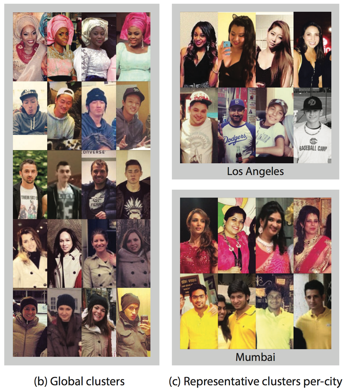](https://user-images.githubusercontent.com/17261080/27176447-d33fc2dc-51c2-11e7-9191-dbf972ee96a1.png)
## Results:
Pretty standard techniques but all patched together to produce interesting visualizations.
|

Visual attribute transfer through deep image analogy
Liao, Jing and Yao, Yuan and Yuan, Lu and Hua, Gang and Kang, Sing Bing
ACM Special Interest Group on computer GRAPHics - 2017 via Local Bibsonomy
Keywords: dblp
Liao, Jing and Yao, Yuan and Yuan, Lu and Hua, Gang and Kang, Sing Bing
ACM Special Interest Group on computer GRAPHics - 2017 via Local Bibsonomy
Keywords: dblp
|
[link]
_Objective:_ Transfer visual attribute (color, tone, texture, and style, etc) between two semantically-meaningful images such as a picture and a sketch. ## Inner workings: ### Image analogy An image analogy A:A′::B:B′ is a relation where: * B′ relates to B in the same way as A′ relates to A * A and A′ are in pixel-wise correspondences * B and B′ are in pixel-wise correspondences In this paper only a source image A and an example image B′ are given, and both A′ and B represent latent images to be estimated. [](https://cloud.githubusercontent.com/assets/17261080/26193907/f080e212-3bb6-11e7-9441-7b255e4219f5.png) ### Dense correspondence In order to find dense correspondences between two images they use features from previously trained CNN (VGG-19) and retrieve all the ReLU layers. The mapping is divided in two sub-mappings that are easier to compute, first a visual attribute transformation and then a space transformation. [](https://cloud.githubusercontent.com/assets/17261080/26194835/03ccd94a-3bba-11e7-93ca-9420d4d96162.png) ## Architecture: The algorithm proceeds as follow: 1. Compute features at each layer for the input image using a pre-trained CNN and initialize feature maps of latent images with coarsest layer. 2. For said layer compute a forward and reverse nearest-neighbor field (NNF, basically an offset field). 3. Use this NNF with the feature of the input current layer to compute the features of the latent images. 4. Upsample the NNF and use it as the initialization for the NNF of the next layer. [](https://cloud.githubusercontent.com/assets/17261080/26195178/35277e0e-3bbb-11e7-82ce-037466314640.png) ## Results: Impressive quality on all type of visual transfer but veryyyyy slow! (~3min on GPUs for one image). [](https://cloud.githubusercontent.com/assets/17261080/26196151/54ef423c-3bbe-11e7-9433-b29be5091fae.png) |
pix2code: Generating Code from a Graphical User Interface Screenshot
Beltramelli, Tony
arXiv e-Print archive - 2017 via Local Bibsonomy
Keywords: dblp
Beltramelli, Tony
arXiv e-Print archive - 2017 via Local Bibsonomy
Keywords: dblp
|
[link]
Generate code from a UI screenshot. _Code:_ [Demo](https://youtu.be/pqKeXkhFA3I) and [code](https://github.com/tonybeltramelli/pix2code) to come. ## Inner-workings: Decomposed the problem in three steps: 1. a computer vision problem of understanding the given scene and inferring the objects present, their identities, positions, and poses. 2. a language modeling problem of understanding computer code and generating syntactically and semantically correct samples. 3. use the solutions to both previous sub-problems by exploiting the latent variables inferred from scene understanding to generate corresponding textual descriptions of the objects represented by these variables. They also introduce a Domain Specific Languages (DSL) for modeling purposes. ## Architecture: * Vision model: usual AlexNet-like architecture * Language model: use onehot encoding for the words in the DSL vocabulary which is then fed into a LSTM * Combined model: LSTM too. [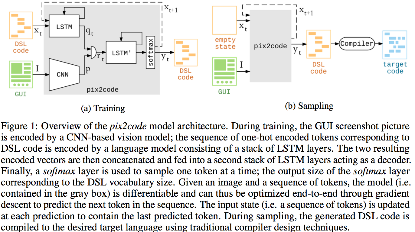](https://user-images.githubusercontent.com/17261080/27221124-c9cadcc6-5287-11e7-9d38-c4234af92912.png) ## Results: Clearly not ready for any serious use but promising results! [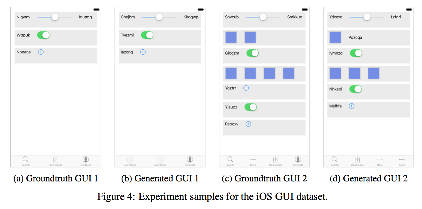](https://user-images.githubusercontent.com/17261080/27222031-0bf8e7de-528b-11e7-896f-cdb410f928c3.png) |
A System for Accessible Artificial Intelligence
Olson, Randal S. and Sipper, Moshe and Cava, William La and Tartarone, Sharon and Vitale, Steven and Fu, Weixuan and Holmes, John H. and Moore, Jason H.
arXiv e-Print archive - 2017 via Local Bibsonomy
Keywords: dblp
Olson, Randal S. and Sipper, Moshe and Cava, William La and Tartarone, Sharon and Vitale, Steven and Fu, Weixuan and Holmes, John H. and Moore, Jason H.
arXiv e-Print archive - 2017 via Local Bibsonomy
Keywords: dblp
|
[link]
_Objective:_ Develop a platform to make AI accessible _Website:_ [here](http://pennai.org/) ## Inner-workings: Platform for AI with deep learning and genetic programming. More focused on biology. ## Architecture: [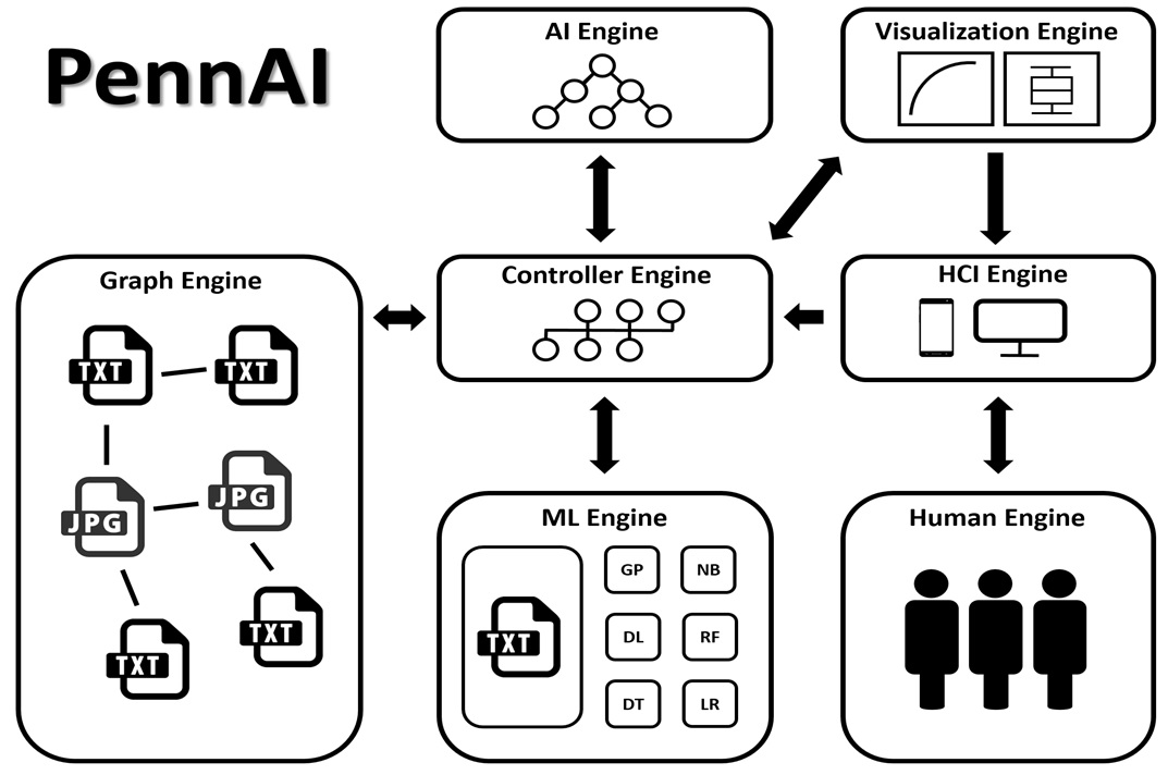](https://user-images.githubusercontent.com/17261080/27690782-8b71f8c8-5ce2-11e7-9d84-77a4dd519e18.jpg) ## Results: Just announced, keep an eye on it. |
Domain Adaptation with Randomized Multilinear Adversarial Networks
Long, Mingsheng and Cao, Zhangjie and Wang, Jianmin and Jordan, Michael I.
arXiv e-Print archive - 2017 via Local Bibsonomy
Keywords: dblp
Long, Mingsheng and Cao, Zhangjie and Wang, Jianmin and Jordan, Michael I.
arXiv e-Print archive - 2017 via Local Bibsonomy
Keywords: dblp
|
[link]
_Objective:_ Perform domain-adaptation by adapting several layers using a randomized representation and not just the final layer thus performing alignment of the joint distribution and not just the marginals.
_Dataset:_ [Office](https://cs.stanford.edu/%7Ejhoffman/domainadapt/) and [ImageCLEF-DA1](http://imageclef.org/2014/adaptation).
## Inner-workings:
Basically an improvement on [RevGrad](https://arxiv.org/pdf/1505.07818.pdf) where instead of using the last embedding layer for the discriminator, a bunch of them is used.
To avoid dimension explosion when using the tensor product of all layers they instead use a randomized multi-linear representation:
[](https://cloud.githubusercontent.com/assets/17261080/26687736/cff20446-46f0-11e7-918e-b60baa10aa67.png)
Where:
* d is the dimension of the embedding (they use 1024)
* R is random matrix for which each element as a null average and variance of 1 (Bernoulli, Gaussian and Uniform are tried)
* z^l is the l-th layer
* ⊙ represents the Hadamard product
In practice they don't use all layers but just the 3-4 last layers for ResNet and AlexNet.
## Architecture:
[](https://cloud.githubusercontent.com/assets/17261080/26687686/acce0d98-46f0-11e7-89d1-15452cbb527e.png)
They use the usual losses for domain adaptation with: - F minimizing the cross-entropy loss for classification and trying to reduce the gap between the distributions (indicated by D). - D maximizing the gap between the distributions.
[](https://cloud.githubusercontent.com/assets/17261080/26687936/8575ff70-46f1-11e7-917d-05129ab190b0.png)
## Results:
Improvement on state-of-the-art results for most tasks in the dataset, very easy to implement with any pre-trained network out of the box.
|
Softmax GAN
Min Lin
arXiv e-Print archive - 2017 via Local arXiv
Keywords: cs.LG, cs.NE
First published: 2017/04/20 (7 years ago)
Abstract: Softmax GAN is a novel variant of Generative Adversarial Network (GAN). The key idea of Softmax GAN is to replace the classification loss in the original GAN with a softmax cross-entropy loss in the sample space of one single batch. In the adversarial learning of $N$ real training samples and $M$ generated samples, the target of discriminator training is to distribute all the probability mass to the real samples, each with probability $\frac{1}{M}$, and distribute zero probability to generated data. In the generator training phase, the target is to assign equal probability to all data points in the batch, each with probability $\frac{1}{M+N}$. While the original GAN is closely related to Noise Contrastive Estimation (NCE), we show that Softmax GAN is the Importance Sampling version of GAN. We futher demonstrate with experiments that this simple change stabilizes GAN training.
more
less
Min Lin
arXiv e-Print archive - 2017 via Local arXiv
Keywords: cs.LG, cs.NE
First published: 2017/04/20 (7 years ago)
Abstract: Softmax GAN is a novel variant of Generative Adversarial Network (GAN). The key idea of Softmax GAN is to replace the classification loss in the original GAN with a softmax cross-entropy loss in the sample space of one single batch. In the adversarial learning of $N$ real training samples and $M$ generated samples, the target of discriminator training is to distribute all the probability mass to the real samples, each with probability $\frac{1}{M}$, and distribute zero probability to generated data. In the generator training phase, the target is to assign equal probability to all data points in the batch, each with probability $\frac{1}{M+N}$. While the original GAN is closely related to Noise Contrastive Estimation (NCE), we show that Softmax GAN is the Importance Sampling version of GAN. We futher demonstrate with experiments that this simple change stabilizes GAN training.
|
[link]
_Objective:_ Replace the usual GAN loss with a softmax croos-entropy loss to stabilize GAN training. _Dataset:_ [CelebA](http://mmlab.ie.cuhk.edu.hk/projects/CelebA.html) ## Inner working: Linked to recent work such as WGAN or Loss-Sensitive GAN that focus on objective functions with non-vanishing gradients to avoid the situation where the discriminator `D` becomes too good and the gradient vanishes. Thus they first introduce two targets for the discriminator `D` and the generator `G`: [](https://cloud.githubusercontent.com/assets/17261080/25347232/767049bc-291a-11e7-906e-c19a92bb7431.png) [](https://cloud.githubusercontent.com/assets/17261080/25347233/7670ff60-291a-11e7-974f-83eb9269d238.png) And then the two new losses: [](https://cloud.githubusercontent.com/assets/17261080/25347275/a303aa0a-291a-11e7-86b4-abd42c83d4a8.png) [](https://cloud.githubusercontent.com/assets/17261080/25347276/a307bc6c-291a-11e7-98b3-cbd7182090cd.png) ## Architecture: They use the DCGAN architecture and simply change the loss and remove the batch normalization and other empirical techniques used to stabilize training. They show that the soft-max GAN is still robust to training. |
Generate To Adapt: Aligning Domains using Generative Adversarial Networks
Sankaranarayanan, Swami and Balaji, Yogesh and Castillo, Carlos D. and Chellappa, Rama
arXiv e-Print archive - 2017 via Local Bibsonomy
Keywords: dblp
Sankaranarayanan, Swami and Balaji, Yogesh and Castillo, Carlos D. and Chellappa, Rama
arXiv e-Print archive - 2017 via Local Bibsonomy
Keywords: dblp
|
[link]
_Objective:_ Use a GAN to learn an embedding invariant from domain shift. _Dataset:_ [MNIST](yann.lecun.com/exdb/mnist/), [SVHN](http://ufldl.stanford.edu/housenumbers/), USPS, [OFFICE](https://cs.stanford.edu/%7Ejhoffman/domainadapt/) and [CFP](http://mukh.com/). ## Architecture: The total network is composed of several sub-networks: 1. `F`, the Feature embedding network that takes as input an image from either the source or target dataset and generate a feature vector. 2. `C`, the Classifier network when the image come from the source dataset. 3. `G`, the Generative network that learns to generate an image similar to the source dataset using an image embedding from `F` and a random noise vector. 4. `D`, the Discriminator network that tries to guess if an image is either from the source or the generative network. `G` and `D` play a minimax game where `D` tries to classify the generated samples as fake and `G` tries to fool `D` by producing examples that are as realistic as possible. The scheme for training the network is the following: [](https://cloud.githubusercontent.com/assets/17261080/25048122/f2a648b6-213a-11e7-93bd-954981bd3838.png) ## Results: Very interesting, the generated image is just a side-product but the overall approach seems to be the state-of-the-art at the time of writing (the paper was published one week ago). |
Neural Episodic Control
Pritzel, Alexander and Uria, Benigno and Srinivasan, Sriram and Badia, Adrià Puigdomènech and Vinyals, Oriol and Hassabis, Demis and Wierstra, Daan and Blundell, Charles
International Conference on Machine Learning - 2017 via Local Bibsonomy
Keywords: dblp
Pritzel, Alexander and Uria, Benigno and Srinivasan, Sriram and Badia, Adrià Puigdomènech and Vinyals, Oriol and Hassabis, Demis and Wierstra, Daan and Blundell, Charles
International Conference on Machine Learning - 2017 via Local Bibsonomy
Keywords: dblp
|
[link]
_Objective:_ Reduce learning time for [DQN](https://deepmind.com/research/dqn/)-type architectures. They introduce a new network element, called DND (Differentiable Neural Dictionary) which is basically a dictionary that uses any key (especially embeddings) and computes the value by using kernel between keys. Plus it's differentiable. ## Architecture: They use basically a network in two steps: 1. A classical CNN network that computes and embedding for every image. 2. A DND for all possible actions (controller input) that stores the embedding as key and estimated reward as value. Also they use a buffer to store all tuples (previous image, action, reward, next image) and for training basic technique is used. [](https://cloud.githubusercontent.com/assets/17261080/24951103/92930022-1f73-11e7-97d2-628e2f4b5a33.png) ## Results: Clearly improves learning speed but in the end other techniques catchup and it gets outperformed. |
Adversarial Discriminative Domain Adaptation
Tzeng, Eric and Hoffman, Judy and Saenko, Kate and Darrell, Trevor
Conference and Computer Vision and Pattern Recognition - 2017 via Local Bibsonomy
Keywords: dblp
Tzeng, Eric and Hoffman, Judy and Saenko, Kate and Darrell, Trevor
Conference and Computer Vision and Pattern Recognition - 2017 via Local Bibsonomy
Keywords: dblp
|
[link]
_Objective:_ Define a framework for Adversarial Domain Adaptation and propose a new architecture as state-of-the-art. _Dataset:_ MNIST, USPS, SVHN and NYUD. ## Inner workings: Subsumes previous work in a generalized framework where designing a new method is now simplified to the space of making three design choices: * whether to use a generative or discriminative base model. * whether to tie or untie the weights. * which adversarial learning objective to use. [](https://cloud.githubusercontent.com/assets/17261080/25138167/15d5e644-245a-11e7-9fb8-636ce4111036.png) ## Architecture: [](https://cloud.githubusercontent.com/assets/17261080/25138526/07848bd0-245b-11e7-94c9-f6ae7ccea76f.png) ## Results: Interesting as the theoretical framework seem to converge with other papers and their architecture improves on previous papers performance even if it's not a huge improvement. |
Cost-Effective Active Learning for Deep Image Classification
Wang, Keze and Zhang, Dongyu and Li, Ya and Zhang, Ruimao and Lin, Liang
IEEE Trans. Circuits Syst. Video Techn. - 2017 via Local Bibsonomy
Keywords: dblp
Wang, Keze and Zhang, Dongyu and Li, Ya and Zhang, Ruimao and Lin, Liang
IEEE Trans. Circuits Syst. Video Techn. - 2017 via Local Bibsonomy
Keywords: dblp
|
[link]
_Objective:_ Specifically adapt Active Learning to Image Classification with deep learning _Dataset:_ [CARC](https://bcsiriuschen.github.io/CARC/) and [Caltech-256](http://authors.library.caltech.edu/7694/) ## Inner-workings: They labels from two sources: * The most informative/uncertain samples are manually labeled using Least confidence, margin sampling and entropy, see [Active Learning Literature Survey](https://github.com/Deepomatic/papers/issues/192). * The other kind is the samples with high prediction confidence that are automatically labelled. They represent the majority of samples. ## Architecture: [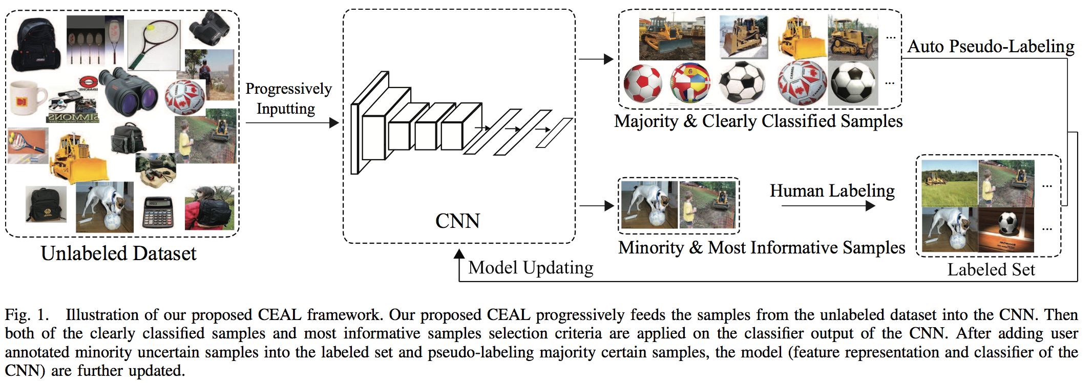](https://user-images.githubusercontent.com/17261080/27691277-d4547196-5ce3-11e7-849c-aadd30d71d68.png) They proceed with the following steps: 1. Initialization: they manually annotate a given number of images for each class in order to pre-trained the network. 2. Complementary sample selection: they fix the network, identity the most uncertain label for manual annotation and automatically annotate the most certain one if their entropy is higher than a given threshold. 3. CNN fine-tuning: they train the network using the whole pool of already labeled data and pseudo-labeled. Then they put all the automatically labeled images back into the unlabelled pool. 4. Threshold updating: as the network gets more and more confident the threshold for auto-labelling is linearly reducing. The idea is that the network gets a more reliable representation and its trustability increases. ## Results: Roughly divide by 2 the number of annotation needed. ⚠️ I don't feel like this paper can be trusted 100% ⚠️ |
Learning from Noisy Large-Scale Datasets with Minimal Supervision
Veit, Andreas and Alldrin, Neil and Chechik, Gal and Krasin, Ivan and Gupta, Abhinav and Belongie, Serge J.
Conference and Computer Vision and Pattern Recognition - 2017 via Local Bibsonomy
Keywords: dblp
Veit, Andreas and Alldrin, Neil and Chechik, Gal and Krasin, Ivan and Gupta, Abhinav and Belongie, Serge J.
Conference and Computer Vision and Pattern Recognition - 2017 via Local Bibsonomy
Keywords: dblp
|
[link]
_Objective:_ Predict labels using a very large dataset with noisy labels and a much smaller (3 orders of magnitude) dataset with human-verified annotations. _Dataset:_ [Open image](https://research.googleblog.com/2016/09/introducing-open-images-dataset.html) ## Architecture: Contrary to other approaches they use the clean labels, the noisy labels but also image features. They basically train 3 networks: 1. A feature extractor for the image. 2. A label Cleaning Network that predicts to learn verified labels from noisy labels + image feature. 3. An image classifier that predicts using just the image. [](https://cloud.githubusercontent.com/assets/17261080/24950258/c4764106-1f70-11e7-82e4-c1111ffc089e.png) ## Results: Overall better performance but not breath-taking improvement: from `AP 83.832 / MAP 61.82` for a NN trained only on labels to `AP 87.67 / MAP 62.38` with their approach. |
Speed/Accuracy Trade-Offs for Modern Convolutional Object Detectors
Huang, Jonathan and Rathod, Vivek and Sun, Chen and Zhu, Menglong and Korattikara, Anoop and Fathi, Alireza and Fischer, Ian and Wojna, Zbigniew and Song, Yang and Guadarrama, Sergio and Murphy, Kevin
Conference and Computer Vision and Pattern Recognition - 2017 via Local Bibsonomy
Keywords: dblp
Huang, Jonathan and Rathod, Vivek and Sun, Chen and Zhu, Menglong and Korattikara, Anoop and Fathi, Alireza and Fischer, Ian and Wojna, Zbigniew and Song, Yang and Guadarrama, Sergio and Murphy, Kevin
Conference and Computer Vision and Pattern Recognition - 2017 via Local Bibsonomy
Keywords: dblp
|
[link]
_Objective:_ Compare several meta-architectures and hyper-parameters in the same framework for easy comparison. ## Architectures: Four meta architectures: 1. R-CNN 2. Faster R-CNN 3. SSD 4. YOLO Architecture (not evaluated in the paper) [](https://cloud.githubusercontent.com/assets/17261080/25746807/5a294360-31a5-11e7-808e-d48497a16cd5.png) ## Results: Very interesting to know which framework to implement or not at first glance. |
Curriculum Q-Learning for Visual Vocabulary Acquisition
Zaidi, Ahmed H. and Moore, Russell and Briscoe, Ted
arXiv e-Print archive - 2017 via Local Bibsonomy
Keywords: dblp
Zaidi, Ahmed H. and Moore, Russell and Briscoe, Ted
arXiv e-Print archive - 2017 via Local Bibsonomy
Keywords: dblp
|
[link]
This paper lays a framework for pedagogically inspired reinforcement learning that can be used to train both students and agents. The paper also draws analogies between theories of language acquisition and those of reinforcement learning. The paper cites work from Elman (1993), Bengio (2009) to show the motivation of curriculum learning and then demonstrates how it can be applied to vocabulary acquisition. There is an interesting reference of zone of proximal development (ZPD) that has not previously been referenced in the context of curriculum learning. ZPD formalises the concept of what we know, what we can learn with some help, and what is beyond our understanding. This is a well motivated concept and can be applied in a way to train agents for any particular task. One of the main reasons for success in AlphaZero by Deepmind was having the optimal opposition, that was neither too strong nor too weak. This allowed the system to use self-play in order to improve learning. There are many parallels between ZPD and optimal opposition such that ZPD can determines what the optimal strength of an opponent should be in order to encourage transfer learning. This idea can also be used to control the discriminator in a GAN. An interesting extension would be to infer the ZPD using a bayesian framework. |
AdaBatch: Adaptive Batch Sizes for Training Deep Neural Networks
Aditya Devarakonda and Maxim Naumov and Michael Garland
arXiv e-Print archive - 2017 via Local arXiv
Keywords: cs.LG, cs.CV, cs.DC, stat.ML, 68T05, , I.2.6; I.5.0
First published: 2017/12/06 (6 years ago)
Abstract: Training deep neural networks with Stochastic Gradient Descent, or its variants, requires careful choice of both learning rate and batch size. While smaller batch sizes generally converge in fewer training epochs, larger batch sizes offer more parallelism and hence better computational efficiency. We have developed a new training approach that, rather than statically choosing a single batch size for all epochs, adaptively increases the batch size during the training process. Our method delivers the convergence rate of small batch sizes while achieving performance similar to large batch sizes. We analyse our approach using the standard AlexNet, ResNet, and VGG networks operating on the popular CIFAR-10, CIFAR-100, and ImageNet datasets. Our results demonstrate that learning with adaptive batch sizes can improve performance by factors of up to 6.25 on 4 NVIDIA Tesla P100 GPUs while changing accuracy by less than 1% relative to training with fixed batch sizes.
more
less
Aditya Devarakonda and Maxim Naumov and Michael Garland
arXiv e-Print archive - 2017 via Local arXiv
Keywords: cs.LG, cs.CV, cs.DC, stat.ML, 68T05, , I.2.6; I.5.0
First published: 2017/12/06 (6 years ago)
Abstract: Training deep neural networks with Stochastic Gradient Descent, or its variants, requires careful choice of both learning rate and batch size. While smaller batch sizes generally converge in fewer training epochs, larger batch sizes offer more parallelism and hence better computational efficiency. We have developed a new training approach that, rather than statically choosing a single batch size for all epochs, adaptively increases the batch size during the training process. Our method delivers the convergence rate of small batch sizes while achieving performance similar to large batch sizes. We analyse our approach using the standard AlexNet, ResNet, and VGG networks operating on the popular CIFAR-10, CIFAR-100, and ImageNet datasets. Our results demonstrate that learning with adaptive batch sizes can improve performance by factors of up to 6.25 on 4 NVIDIA Tesla P100 GPUs while changing accuracy by less than 1% relative to training with fixed batch sizes.
|
[link]
**TL;DR**: You can increase batch size in advanced phases of training without hurting accuracy and gaining some speedup. You should multiply the learning rate by the same value you multiplied batch size. **Long version**: Authors propose to increase batch size gradually, starting with a small batch size $r$, and then progressively increase the batch size while adapting the learning rate $\alpha$ so that the ratio $\alpha/r$ remains constant (without taking in account scheduled LR reduce). In this paper, they double the batch size by schedule. At the same time, learning rate is decayed and then multiplied by 2 to compensate batch size increase: if in baseline lr is multiplied by $0.375$, it is multiplied by $0.75$ now. The experiments on CIFAR-100 dataset show that the gradual increase of batch size allows to converge to the same values as constant small batch size. However, bigger batches allow faster training, providing $\times 1.5$ speedup on AlexNet, and around $\times 1.2$ speedup on ResNet and VGG, for both forward and backward passes on single GPU. On multiple GPUs the approach allows to further increase batchsize. On fortunate setups authors manage to get up to $\times 1.6$ speedup compared to constant batch size equal to initial value, while the error is almost unchanged. For bigger batch sizes lr warmup is used. For ImageNet, same behavior is shown for accuracy: gradual increase of batch size converges to same values as setup with initial batch size. Since authors haven't access to a system capable of processing large batches on ImageNet, no performance results are reported. |

A Regularized Framework for Sparse and Structured Neural Attention.
Vlad Niculae and Mathieu Blondel
Neural Information Processing Systems Conference - 2017 via Local dblp
Keywords:
Vlad Niculae and Mathieu Blondel
Neural Information Processing Systems Conference - 2017 via Local dblp
Keywords:
|
[link]
The idea in this paper is to develop a version of attention that will incorporate similarity in neighboring bins. This aligned with the work \cite{conf/icml/BeckhamP17} which presented a different approach to deal with consistency between classes of predictions.

In this work the closed form softmax function is replaced by a small optimization problem with this regularizer:

$$ +\lambda \sum_{i=1}^{d-1} |y_{i+1}-y_i|$$

Because of this, many of the neighboring probabilities are exactly the same resulting in attention that can be seen as blocks.

https://i.imgur.com/oue0x4V.png

Poster:
https://i.imgur.com/gclMjzR.png
|

Geometric Deep Learning: Going beyond Euclidean data
Bronstein, Michael M. and Bruna, Joan and LeCun, Yann and Szlam, Arthur and Vandergheynst, Pierre
IEEE Signal Process. Mag. - 2017 via Local Bibsonomy
Keywords: dblp
Bronstein, Michael M. and Bruna, Joan and LeCun, Yann and Szlam, Arthur and Vandergheynst, Pierre
IEEE Signal Process. Mag. - 2017 via Local Bibsonomy
Keywords: dblp
|
[link]
This paper surveys progress on adapting deep learning techniques to non-Euclidean data and suggests future directions. One of the strengths (and weaknesses) of deep learning--specifically exploited by convolutional neural networks--is that the data is assumed to exhibit translation invariance/equivariance and invariance to local deformations. Hence, long-range dependencies can be learned with multi-scale, hierarchical techniques where spatial resolution is reduced. However, this means that any information about the data that can't be learned when spatial resolution is reduced can get lost (I believe that residual networks aim to address this by the skip connections that are able to learn an identity operation; also, in computer vision, multi-scale versions of the data are often fed to CNNs). Key areas where this assumption about the data appears to be true is computer vision and speech recognition.

#### Some quick background

The *Laplacian*, a self-adjoint (symmetric) positive semi-definite operator, which is defined for smooth manifolds and graphs in this paper, can be thought of as the difference between the local average of a function around a point and the value of the function at the point itself. It's generally defined as $\triangle = -\text{div} \nabla$. When discretizing a continuous, smooth manifold with a *mesh*, note that the graph Laplacian might not converge to the continuous Laplacian operator with increasing sampling density. To be consistent, need to create a triangular mesh, i.e., represent the manifold as a polyhedral surface.

### Spectral methods

Fourier analysis on non-Euclidean domains is possible by considering the eigendecomposition of the Laplacian operator. A possible transformation of the Convolution Theorem to functions on manifolds and graphs is discussed, but is noted as not being shift-invariant.

The Spectral CNN can be defined by introducing a spectral convolutional layer acting on the vertices of the graph and using filters in the frequency domain and the eigenvectors of the Laplacian. However, the spectral filter coefficients will be dependent on the particular eigenvectors (basis) - domain dependency == bad for generalization!

The non-Euclidean analogy of pooling is *graph coarsening*- only a fraction of the vertices of the graph are retained. Strided convolutions can be generalized to the spectral construction by only keeping the low-frequency components - must recompute the graph Laplacian after applying the nonlinearity in the spatial domain, however.

Performing matrix multiplications on the eigendecomposition of the Laplacian is expensive!

### Spectrum-free Methods

**A polynomial of the Laplacian acts as a polynomial on the eigenvalues**. ChebNet (Defferrard et al.) and Graph Convolutional Networks (Kipf et al.) boil down to applying simple filters acting on the r- or 1-hop neighborhood of the graph in the spatial domain.

Some examples of generalizations of CNNs that define weighting functions for a locally Euclidean coordinate system around a point on a manifold are the
  * Geodesic CNN
  * Anisotropic CNN
  * Mixture Model network (MoNet)


#### What problems are being solved with these methods?

* Ranking and community detection on social networks
* Recommender systems
* 3D geometric data in Computer Vision/Graphics
    * Shape classification
    * Feature correspondence for 3D shapes
* Behavior of N-particle systems (particle physics, LHC)
* Molecule design
* Medical imaging

### Open Problems

* *Generalization* spectral analogues of convolution learned on one graph cannot be readily applied to other ones (domain dependency). Spatial methods generalize across different domains, but come with their own subtleties
* *Time-varying domains*
* *Directed graphs* non-symmetric Laplacian that do not have orthogonal eigendecompositions for interpretable spectral-domain constructions
* *Synthesis problems* generative models
* *Computation* extending deep learning frameworks for non-Euclidean data
|

Triangle Generative Adversarial Networks
Zhe Gan and Liqun Chen and Weiyao Wang and Yunchen Pu and Yizhe Zhang and Hao Liu and Chunyuan Li and Lawrence Carin
arXiv e-Print archive - 2017 via Local arXiv
Keywords: cs.LG, stat.ML
First published: 2017/09/19 (6 years ago)
Abstract: A Triangle Generative Adversarial Network ($\Delta$-GAN) is developed for semi-supervised cross-domain joint distribution matching, where the training data consists of samples from each domain, and supervision of domain correspondence is provided by only a few paired samples. $\Delta$-GAN consists of four neural networks, two generators and two discriminators. The generators are designed to learn the two-way conditional distributions between the two domains, while the discriminators implicitly define a ternary discriminative function, which is trained to distinguish real data pairs and two kinds of fake data pairs. The generators and discriminators are trained together using adversarial learning. Under mild assumptions, in theory the joint distributions characterized by the two generators concentrate to the data distribution. In experiments, three different kinds of domain pairs are considered, image-label, image-image and image-attribute pairs. Experiments on semi-supervised image classification, image-to-image translation and attribute-based image generation demonstrate the superiority of the proposed approach.
more
less
Zhe Gan and Liqun Chen and Weiyao Wang and Yunchen Pu and Yizhe Zhang and Hao Liu and Chunyuan Li and Lawrence Carin
arXiv e-Print archive - 2017 via Local arXiv
Keywords: cs.LG, stat.ML
First published: 2017/09/19 (6 years ago)
Abstract: A Triangle Generative Adversarial Network ($\Delta$-GAN) is developed for semi-supervised cross-domain joint distribution matching, where the training data consists of samples from each domain, and supervision of domain correspondence is provided by only a few paired samples. $\Delta$-GAN consists of four neural networks, two generators and two discriminators. The generators are designed to learn the two-way conditional distributions between the two domains, while the discriminators implicitly define a ternary discriminative function, which is trained to distinguish real data pairs and two kinds of fake data pairs. The generators and discriminators are trained together using adversarial learning. Under mild assumptions, in theory the joint distributions characterized by the two generators concentrate to the data distribution. In experiments, three different kinds of domain pairs are considered, image-label, image-image and image-attribute pairs. Experiments on semi-supervised image classification, image-to-image translation and attribute-based image generation demonstrate the superiority of the proposed approach.
|
[link]
This paper introduces triangle-GAN ($\triangle$-GAN) that aims at cross-domain joint distribution matching: The model is shown below

https://i.imgur.com/boIDOMu.png

Having two domains of data $x$ and $y$, there are two generators:

1- $G_x(y)$ which takes $y$ and generates $\tilde{x}$

2- $G_y(x)$ which takes $x$ and generates $\tilde{y}$

There are two discriminators in the model:

1- $D_1 (x,y)$ a discriminator that distinguishes between $(x, y)$ and either of $(x, \tilde{y})$ or $(\tilde{x}, y)$.

2- $D_2 (x,y)$ a discriminator that distinguishes between $(x, \tilde{y})$ and $(\tilde{x}, y)$.

The second discriminator is ALI and can be used on un-paired sets of data.
The first discriminator is equivalent to a conditional discriminator where the true paired data $(x, y)$ is compared to either $(x, \tilde{y})$ or $(\tilde{x}, y)$, where one element in the pair is sampled. This discriminator needs paired $(x, y)$ data for training.

This model can be used for semi-supervised settings, where a small set of paired data is provided. In this paper it is used for:

-  semi-supervised image classification, where a small subset of CIFAR10 is labelled. $x$ and $y$ are images and class labels here.

- image to image translation on edge2shoes dataset, where only a subset of dataset is paired.

- attribute conditional image generation where $x$ and $y$ domains are image and attributes. CelebA and COCO datasets are used here. In one experiment test-set images are projected to attributes and then given those attributes new images are generated:

On celebA:
https://i.imgur.com/EX5tDZ0.png

On COCO:
https://i.imgur.com/GRpvjGx.png

In another experiment some attributes are chosen (as samples shown below in the first row with different noise) and then another feature is added (using the same noise) to generate the samples in the second row:
 https://i.imgur.com/KeHL8Ye.png

The triangle gan demonstrates improved performance compared to triple gan in the experiments shown in the paper. It has been also compared with Disco gan (a model that can be trained on un-paired data) and shows improved performance when some percentage of paired data is provided. In an experiment they pair each MNIST digit with its transposed (as $x$, $y$ pairs). Disco-GAN cannot learn correct mapping between them, while triangle-GAN can learn correct mapping since it leverages paired data.

https://i.imgur.com/Vz9Zfhu.png

In general this model is a useful approach for semi-supervised cross-domain matching and can leverage un-paired data (using ALI) as well as paired data (using conditional discriminator).
|
Fader Networks: Manipulating Images by Sliding Attributes
Lample, Guillaume and Zeghidour, Neil and Usunier, Nicolas and Bordes, Antoine and Denoyer, Ludovic and Ranzato, Marc'Aurelio
arXiv e-Print archive - 2017 via Local Bibsonomy
Keywords: dblp
Lample, Guillaume and Zeghidour, Neil and Usunier, Nicolas and Bordes, Antoine and Denoyer, Ludovic and Ranzato, Marc'Aurelio
arXiv e-Print archive - 2017 via Local Bibsonomy
Keywords: dblp
|
[link]
This paper aims at changing the attributes of a face, without manipulating other aspects of the image, such as add/remove glasses, make a person young/old, changed the gender, and hence the name Fader Networks, similar to sliders of audio mixing tools that can change a value linearly to increase/decrease a feature. The model is shown below: https://i.imgur.com/fntPmNu.png An image $x$ is passed to the encoder and the output of the encoder $E(x)$ is passed to the discriminator to distinguish whether a feature $y$ is in the latent space or not. The encoded features $E(x)$ and the feature $y$ is passed to the decoder to reconstruct the image $D(E(x))$. The AE therefore has two loss: 1- The reconstruction loss between $x$ and $D(E(x))$, and 2- The gan loss to fool the discriminator on the feature $y$ in the encoded space $E(x)$. The discriminator tries to distinguish whether a feature $y$ is in the encoded space $E(x)$ or not, while the encoder tries to fool the discriminator. This process leads to removal of the feature $y$ from the $E(x)$ by encoder. The encoded feature $E(x)$ therefore does not have any information on $y$. However, since the decoder needs to reconstruct the same input image, $E(x)$ has to maintain all information, except the feature $y$ and the decoder should get the feature $y$ from the input of the decoder. The model is trained on binary $y$ features such as: male/female, young/old, glasses Yes/No, mouth open Yes/No, eyes open Yes/No (some samples from test set below): https://i.imgur.com/bj9wu6B.png At test time, they can change the features continuously and show transition in the features: https://i.imgur.com/XUD3ZTu.png The performance of the model is measured using mechanical turks on two metrics: Naturalness of the images and the accuracy of swapping features on the image. In both FadNet shows better results compared to IcGAN, and FadNet shows very good results on accuracy, however on naturalness the performance drops when some features are swapped. On Flowers dataset, FadNet can change colors of the flowers: https://i.imgur.com/7nvBSEY.png I find the following positive aspects about FadNet: 1- It can change some features while maintaining other features of the image such as identity of the person, background information, etc. 2- The model does not need paired data. In some cases it is impossible to gather paired data (e.g. male/female) or very difficult (young/old). 3- The gan loss is used to remove a feature in the latent space, where that feature can be later specified for reconstruction by decoder. Since GAN is applied to latent space, it can be used to remove features on the data that is discrete (where direct usage of disc on those data is not trivial). I think these aspects need further work for improvement: - When multiple features are changed the blurriness of the image shows up: https://i.imgur.com/LD5cVbg.png When only one feature changes the blurriness affect is much less, despite the fact that they use L2-loss for AE reconstruction. I guess also using a high resolution of 256*256 helps make the bluriness of the images less noticeable. - The model should be first trained only on AE (no gan loss) and then the gan loss in AE is linearly increased to remove a feature. So, it requires a bit of care in training it properly. Overall, I find it an interesting paper on how to change a feature in an image when one wants to keep other features unchanged. |
Crossing Nets: Dual Generative Models with a Shared Latent Space for Hand Pose Estimation
Chengde Wan and Thomas Probst and Luc Van Gool and Angela Yao
arXiv e-Print archive - 2017 via Local arXiv
Keywords: cs.CV
First published: 2017/02/11 (7 years ago)
Abstract: State-of-the-art methods for 3D hand pose estimation from depth images require large amounts of annotated training data. We propose to model the statistical relationships of 3D hand poses and corresponding depth images using two deep generative models with a shared latent space. By design, our architecture allows for learning from unlabeled image data in a semi-supervised manner. Assuming a one-to-one mapping between a pose and a depth map, any given point in the shared latent space can be projected into both a hand pose and a corresponding depth map. Regressing the hand pose can then be done by learning a discriminator to estimate the posterior of the latent pose given some depth map. To improve generalization and to better exploit unlabeled depth maps, we jointly train a generator and a discriminator. At each iteration, the generator is updated with the back-propagated gradient from the discriminator to synthesize realistic depth maps of the articulated hand, while the discriminator benefits from an augmented training set of synthesized and unlabeled samples. The proposed discriminator network architecture is highly efficient and runs at 90 FPS on the CPU with accuracies comparable or better than state-of-art on 3 publicly available benchmarks.
more
less
Chengde Wan and Thomas Probst and Luc Van Gool and Angela Yao
arXiv e-Print archive - 2017 via Local arXiv
Keywords: cs.CV
First published: 2017/02/11 (7 years ago)
Abstract: State-of-the-art methods for 3D hand pose estimation from depth images require large amounts of annotated training data. We propose to model the statistical relationships of 3D hand poses and corresponding depth images using two deep generative models with a shared latent space. By design, our architecture allows for learning from unlabeled image data in a semi-supervised manner. Assuming a one-to-one mapping between a pose and a depth map, any given point in the shared latent space can be projected into both a hand pose and a corresponding depth map. Regressing the hand pose can then be done by learning a discriminator to estimate the posterior of the latent pose given some depth map. To improve generalization and to better exploit unlabeled depth maps, we jointly train a generator and a discriminator. At each iteration, the generator is updated with the back-propagated gradient from the discriminator to synthesize realistic depth maps of the articulated hand, while the discriminator benefits from an augmented training set of synthesized and unlabeled samples. The proposed discriminator network architecture is highly efficient and runs at 90 FPS on the CPU with accuracies comparable or better than state-of-art on 3 publicly available benchmarks.
|
[link]
This paper merges a GAN and VAE to improve pose estimation on depth hand images.

They used paired data (where both depth image ($x$) and pose ($y$) is provided) and merge that with unlabelled data where only depth image ($x$) is given. The model is shown below:
https://i.imgur.com/BvjZekU.png

The VAE model takes $y$ and projects it to latent space ($z_y$) using encoder and then reconstructs it back to $\bar y$.

Ali is used to map between latent space of VAE $z_y$ and the latent space of GAN $z_x$.
The depth image synthesizer takes $z_x$ and generates a depth image $\bar x$.

The Discriminator does three tasks:

1-$L_{gan}$: distinguishing between true ($x$) and generated sample ($\bar x$).

2- $L_{pos}$: predicting the pose of the true depth image $x$.

3: $L_{smo}$: a smoothing loss to enforce the difference between two latent spaces in the generator and the ones predicted by discriminator to be the same (see below for more details).

$\textbf{Here is how the data flows and losses are defined:}$ Given a pair of labelled data $(x,y)$, the pose $y$ is projected to latent space $z_y$, then projected back to estimate pose $\bar y$.
Using VAE model, a reconstruction loss $L_{recons}$ is defined on pose.
Using Ali, the latent variable $z_y$ is projected to $z_x$ and then the depth image $\bar{x}$ is generated $\bar{x} = Gen(Ali({z_y}))$. A reconstruction loss between x and $\bar{x}$ is defined (d_{self}).
A random noise is samples from pose latent space ($\hat{z_y}$) and projected to a depth map using $\hat{x} = Gen(Ali(\hat{z_y}))$. Discriminator then takes $x$ and $\hat{x}$. It estimates pose on $x$ using $L_{pos}$. It also distinguishes between $x$ and $\hat{x}$ with $L_{gan}$. Finally, it measures the $x$ and $\hat{x}$'s latent space difference $smo(x, \hat x)$, which should be similar to the distance between $z_y$ and $\hat{z_y}$, so the smo-loss is: $L_{smo} = || smo(x, \hat x) - (z_y - \hat{z_y})||^2 + d_{self}$.


In general the the VAE model and the depth image synthesizer can be considered as the Generator of the network. The total loss can be written as:

$L_G = L_{recons} + L_{smo} - L_{gan}\\$
$L_D = L_{pos} + L_{smo} - L_{gan}\\$

The generator loss contains pose reconstruction, smo-loss, and gan loss on generated depth maps.
The discriminator loss contains pose estimation loss, smo-loss, and gan loss on distinguishing fake and real depth images.

Note that in the gen and disc losses all except the gan loss need paired data and the un-labelled data can be used for only gan-loss. However, the unlabelled data would train the lowest layers of the disc (for pose estimation) and the image synthesis part of gen. But for pose estimation (the final target of the paper), training the VAE model, and also mapping between VAE and GAN using Ali, labelled data should be provided. Also note that $ L_{smo}$ trains both generator and discriminator parameters.

In terms of performance the model improves the results on partially labelled data. On fully labelled data it shows either improvement or comparable results w.r.t to previous models. I find the strongest aspect of the paper in semi-supervised learning where smaller portion of labelled data is provided, However, due to the way parameters are binded together, the model needs some labelled data to train the model completely.
|
Reparameterizing the Birkhoff Polytope for Variational Permutation Inference
Scott W. Linderman and Gonzalo E. Mena and Hal Cooper and Liam Paninski and John P. Cunningham
arXiv e-Print archive - 2017 via Local arXiv
Keywords: stat.ML
First published: 2017/10/26 (6 years ago)
Abstract: Many matching, tracking, sorting, and ranking problems require probabilistic reasoning about possible permutations, a set that grows factorially with dimension. Combinatorial optimization algorithms may enable efficient point estimation, but fully Bayesian inference poses a severe challenge in this high-dimensional, discrete space. To surmount this challenge, we start with the usual step of relaxing a discrete set (here, of permutation matrices) to its convex hull, which here is the Birkhoff polytope: the set of all doubly-stochastic matrices. We then introduce two novel transformations: first, an invertible and differentiable stick-breaking procedure that maps unconstrained space to the Birkhoff polytope; second, a map that rounds points toward the vertices of the polytope. Both transformations include a temperature parameter that, in the limit, concentrates the densities on permutation matrices. We then exploit these transformations and reparameterization gradients to introduce variational inference over permutation matrices, and we demonstrate its utility in a series of experiments.
more
less
Scott W. Linderman and Gonzalo E. Mena and Hal Cooper and Liam Paninski and John P. Cunningham
arXiv e-Print archive - 2017 via Local arXiv
Keywords: stat.ML
First published: 2017/10/26 (6 years ago)
Abstract: Many matching, tracking, sorting, and ranking problems require probabilistic reasoning about possible permutations, a set that grows factorially with dimension. Combinatorial optimization algorithms may enable efficient point estimation, but fully Bayesian inference poses a severe challenge in this high-dimensional, discrete space. To surmount this challenge, we start with the usual step of relaxing a discrete set (here, of permutation matrices) to its convex hull, which here is the Birkhoff polytope: the set of all doubly-stochastic matrices. We then introduce two novel transformations: first, an invertible and differentiable stick-breaking procedure that maps unconstrained space to the Birkhoff polytope; second, a map that rounds points toward the vertices of the polytope. Both transformations include a temperature parameter that, in the limit, concentrates the densities on permutation matrices. We then exploit these transformations and reparameterization gradients to introduce variational inference over permutation matrices, and we demonstrate its utility in a series of experiments.
|
[link]
This paper directly relies on understanding [Gumbel-Softmax][gs] ([Concrete][]) sampling.

The place to start thinking about this paper is in terms of a distribution over possible permutations. You could, for example, have a categorical distribution over all the permutation matrices of a given size. Of size 2 this is easy:

```
p(M)   0.1    0.9

M:     1, 0   0, 1
       0, 1   1, 0
```

You could apply the Gumbel-Softmax trick to this, and other selections of permutation matrices in small dimensions, but the number of possible permutations grows factorially with the dimension. If you want to infer the order of $100$ items, you now have a categorical over $100!$ variables, and you can't even store that number in floating point.

By breaking up and applying a normalised weight to each permutation matrix, we are effectively doing a [Naive Birkhoff-Von Neumann decomposition][naive] to return a sample from the space of Doubly Stochastic matrices. This paper proposes *much* more efficient ways to sample from this space in a way that is amenable to stochastic variational (read *SGD*) methods, such that they have an experiment working with permutations of 278 variables.

There are two ingredients to a good stochastic variational recipe:

1. A differentiable sampling method; for example (most famously): $x = \mu + \sigma \epsilon \text{ where } \epsilon \sim \mathcal{N}(0,1)$
2. A density over this sampling distribution; in the preceding example: $\mathcal{N}(\mu, \sigma)$

This paper presents two recipes: Stick-breaking transformations and Rounding towards permutation matrices.

Stick-breaking
--------------------

[Shakir Mohamed wrote a good blog post on stick-breaking methods.][sticks]

One problem, which you could guess from the categorical-over-permutations example above, is we can't possibly store a probability for each permutation matrix ($N!$ is a lot of numbers to store). Stick-breaking gives us another way to represent these probabilities implicitly through $B \in [0,1]^{(N-1)\times (N-1)}$. The row `x` gets recursively broken up like this:

```
    B_11    B_12*(1-x[:1].sum())     1-x[:2].sum()
x: |-------|------------------------|---------------------|
    x[0]    x[1]                     x[2]
    <---------------------------------------------------->
                               1.0
```

For two dimensions, this becomes a little more complicated (and is actually a novel part of this paper) so I'll just refer you to the paper and say: *this is also possible in two dimensions*.

OK, so now to sample from the distribution of Doubly Stochastic matrices, you just need to sample $(N-1) \times (N-1)$ values in the range $[0,1]$. The authors sample a Gaussian and pass it through a sigmoid. Along with a temperature parameter, the values get pushed closer to 0 or 1 and the result is a permutation matrix.

To get the density, the authors *appear to* (this would probably be annoying in high dimensions) automatically differentiate through the $N^2$ steps of the stick-breaking transformation to get the Jacobian and use change of variables.

Rounding
-------------

This method is more idiosyncratic, so I'll just copy the steps straight from the paper:

> 1. Input $Z \in R^{N \times N} $, $M \in R_+^{N \times N}$, and $V \in  R_+^{N \times N}$;
> 2. Map $M \to \tilde{M}$, a point in the Birkhoff polytope, using the [Sinkhorn-Knopp algorithm][sk];
> 3. Set $\Psi = \tilde{M} + V \odot Z$ where $\odot$ denotes elementwise multiplication;
> 4. Find $\text{round}(\Psi)$, the nearest permutation matrix to $\Psi$, using the [Hungarian algorithm][ha];
> 5. Output $X = \tau \Psi + (1- \tau)\text{round}(\Psi)$.

So you can just schedule $\tau \to 0$ and you'll be moving your distribution to be a distribution over permutation matrices.

The big problem with this is we *can't easily get the density*. Step 4 is not differentiable. However, the authors argue the function is still piecewise-linear so we can just get around this. Once they've done that, it's possible to evaluate the density by change of variables again.

Results
----------

On a synthetic permutation matching problem, the rounding method gets a better match to the true posterior (the synthetic problem is small enough to enumerate the true posterior). It also performs better than competing methods on a real matching problem; matching the activations in neurons of C. Elegans to the location of neurons in the known connectome.

[sticks]: http://blog.shakirm.com/2015/12/machine-learning-trick-of-the-day-6-tricks-with-sticks/
[naive]: https://en.wikipedia.org/wiki/Doubly_stochastic_matrix#Birkhoff_polytope_and_Birkhoff.E2.80.93von_Neumann_theorem
[gs]: http://www.shortscience.org/paper?bibtexKey=journals/corr/JangGP16
[concrete]: http://www.shortscience.org/paper?bibtexKey=journals/corr/1611.00712
[sk]: https://en.wikipedia.org/wiki/Sinkhorn%27s_theorem#Sinkhorn-Knopp_algorithm
[ha]: https://en.wikipedia.org/wiki/Hungarian_algorithm
|

Introspective Generative Modeling: Decide Discriminatively
Justin Lazarow and Long Jin and Zhuowen Tu
arXiv e-Print archive - 2017 via Local arXiv
Keywords: cs.CV, cs.LG, cs.NE
First published: 2017/04/25 (7 years ago)
Abstract: We study unsupervised learning by developing introspective generative modeling (IGM) that attains a generator using progressively learned deep convolutional neural networks. The generator is itself a discriminator, capable of introspection: being able to self-evaluate the difference between its generated samples and the given training data. When followed by repeated discriminative learning, desirable properties of modern discriminative classifiers are directly inherited by the generator. IGM learns a cascade of CNN classifiers using a synthesis-by-classification algorithm. In the experiments, we observe encouraging results on a number of applications including texture modeling, artistic style transferring, face modeling, and semi-supervised learning.
more
less
Justin Lazarow and Long Jin and Zhuowen Tu
arXiv e-Print archive - 2017 via Local arXiv
Keywords: cs.CV, cs.LG, cs.NE
First published: 2017/04/25 (7 years ago)
Abstract: We study unsupervised learning by developing introspective generative modeling (IGM) that attains a generator using progressively learned deep convolutional neural networks. The generator is itself a discriminator, capable of introspection: being able to self-evaluate the difference between its generated samples and the given training data. When followed by repeated discriminative learning, desirable properties of modern discriminative classifiers are directly inherited by the generator. IGM learns a cascade of CNN classifiers using a synthesis-by-classification algorithm. In the experiments, we observe encouraging results on a number of applications including texture modeling, artistic style transferring, face modeling, and semi-supervised learning.
|
[link]
In this work they take a different approach to the GAN model \cite{1406.2661}. In the traditionally GAN model a neural network is trained to up-sample from random noise in a feed forward fashion to generate samples from the data distribution.

This work instead iteratively permutes an image of random noise similar to Artistic Style Transfer \cite{1508.06576}.  The image is permuted in order to fool a set of discriminators. To obtain the set of discriminators each is trained starting from random noise until some max $t$ step.


1. At first a discriminator is trained to discriminate between the true data and random noise .
2. Images is then permuted using gradients which aim to fool the discriminator and included in the data distribution as a negative example.
3. The discriminator is trained on the true data + random noise + fake data from the previous steps

The images generated at each step are shown below:

https://i.imgur.com/kp575s8.png

After being trained the model is able to generate a sample by iterating over each trained discriminator and applying gradient updates on from random noise. For this storing only the weights of the discriminators is required.

Poster from ICCV2017:
https://i.imgur.com/vYSSdZx.png
|
BEGAN: Boundary Equilibrium Generative Adversarial Networks
David Berthelot and Thomas Schumm and Luke Metz
arXiv e-Print archive - 2017 via Local arXiv
Keywords: cs.LG, stat.ML
First published: 2017/03/31 (7 years ago)
Abstract: We propose a new equilibrium enforcing method paired with a loss derived from the Wasserstein distance for training auto-encoder based Generative Adversarial Networks. This method balances the generator and discriminator during training. Additionally, it provides a new approximate convergence measure, fast and stable training and high visual quality. We also derive a way of controlling the trade-off between image diversity and visual quality. We focus on the image generation task, setting a new milestone in visual quality, even at higher resolutions. This is achieved while using a relatively simple model architecture and a standard training procedure.
more
less
David Berthelot and Thomas Schumm and Luke Metz
arXiv e-Print archive - 2017 via Local arXiv
Keywords: cs.LG, stat.ML
First published: 2017/03/31 (7 years ago)
Abstract: We propose a new equilibrium enforcing method paired with a loss derived from the Wasserstein distance for training auto-encoder based Generative Adversarial Networks. This method balances the generator and discriminator during training. Additionally, it provides a new approximate convergence measure, fast and stable training and high visual quality. We also derive a way of controlling the trade-off between image diversity and visual quality. We focus on the image generation task, setting a new milestone in visual quality, even at higher resolutions. This is achieved while using a relatively simple model architecture and a standard training procedure.
|
[link]
* [Detailed Summary](https://blog.heuritech.com/2017/04/11/began-state-of-the-art-generation-of-faces-with-generative-adversarial-networks/)
* [Tensorflow implementation](https://github.com/carpedm20/BEGAN-tensorflow)
### Summary
* They suggest a GAN algorithm that is based on an autoencoder with Wasserstein distance.
* Their method generates highly realistic human faces.
* Their method has a convergence measure, which reflects the quality of the generates images.
* Their method has a diversity hyperparameter, which can be used to set the tradeoff between image diversity and image quality.
### How
* Like other GANs, their method uses a generator G and a discriminator D.
* Generator
* The generator is fairly standard.
* It gets a noise vector `z` as input and uses upsampling+convolutions to generate images.
* It uses ELUs and no BN.
* Discriminator
* The discriminator is a full autoencoder (i.e. it converts input images to `8x8x3` tensors, then reconstructs them back to images).
* It has skip-connections from the `8x8x3` layer to each upsampling layer.
* It also uses ELUs and no BN.
* Their method now has the following steps:
1. Collect real images `x_real`.
2. Generate fake images `x_fake = G(z)`.
3. Reconstruct the real images `r_real = D(x_real)`.
4. Reconstruct the fake images `r_fake = D(x_fake)`.
5. Using an Lp-Norm (e.g. L1-Norm), compute the reconstruction loss of real images `d_real = Lp(x_real, r_real)`.
6. Using an Lp-Norm (e.g. L1-Norm), compute the reconstruction loss of fake images `d_fake = Lp(x_fake, r_fake)`.
7. The loss of D is now `L_D = d_real - d_fake`.
8. The loss of G is now `L_G = -L_D`.
* About the loss
* `r_real` and `r_fake` are really losses (e.g. L1-loss or L2-loss). In the paper they use `L(...)` for that. Here they are referenced as `d_*` in order to avoid confusion.
* The loss `L_D` is based on the Wasserstein distance, as in WGAN.
* `L_D` assumes, that the losses `d_real` and `d_fake` are normally distributed and tries to move their mean values. Ideally, the discriminator produces very different means for real/fake images, while the generator leads to very similar means.
* Their formulation of the Wasserstein distance does not require K-Lipschitz functions, which is why they don't have the weight clipping from WGAN.
* Equilibrium
* The generator and discriminator are at equilibrium, if `E[r_fake] = E[r_real]`. (That's undesirable, because it means that D can't differentiate between fake and real images, i.e. G doesn't get a proper gradient any more.)
* Let `g = E[r_fake] / E[r_real]`, then:
* Low `g` means that `E[r_fake]` is low and/or `E[r_real]` is high, which means that real images are not as well reconstructed as fake images. This means, that the discriminator will be more heavily trained towards reconstructing real images correctly (as that is the main source of error).
* High `g` conversely means that real images are well reconstructed (compared to fake ones) and that the discriminator will be trained more towards fake ones.
* `g` gives information about how much G and D should be trained each (so that none of the two overwhelms the other).
* They introduce a hyperparameter `gamma` (from interval `[0,1]`), which reflects the target value of the balance `g`.
* Using `gamma`, they change their losses `L_D` and `L_G` slightly:
* `L_D = d_real - k_t d_fake`
* `L_G = r_fake`
* `k_t+1 = k_t + lambda_k (gamma d_real - d_fake)`.
* `k_t` is a control term that controls how much D is supposed to focus on the fake images. It changes with every batch.
* `k_t` is clipped to `[0,1]` and initialized at `0` (max focus on reconstructing real images).
* `lambda_k` is like the learning rate of the control term, set to `0.001`.
* Note that `gamma d_real - d_fake = 0 <=> gamma d_real = d_fake <=> gamma = d_fake / d_real`.
* Convergence measure
* They measure the convergence of their model using `M`:
* `M = d_real + |gamma d_real - d_fake|`
* `M` goes down, if `d_real` goes down (D becomes better at autoencoding real images).
* `M` goes down, if the difference in reconstruction error between real and fake images goes down, i.e. if G becomes better at generating fake images.
* Other
* They use Adam with learning rate 0.0001. They decrease it by a factor of 2 whenever M stalls.
* Higher initial learning rate could lead to model collapse or visual artifacs.
* They generate images of max size 128x128.
* They don't use more than 128 filters per conv layer.
### Results
* NOTES:
* Below example images are NOT from generators trained on CelebA. They used a custom dataset of celebrity images. They don't show any example images from the dataset. The generated images look like there is less background around the faces, making the task easier.
* Few example images. Unclear how much cherry picking was involved. Though the results from the tensorflow example (see like at top) make it look like the examples are representative (aside from speckle-artifacts).
* No LSUN Bedrooms examples. Human faces are comparatively easy to generate.
* Example images at 128x128:
* 
* Effect of changing the target balance `gamma`:
* 
* High gamma leads to more diversity at lower quality.
* Interpolations:
* 
* Convergence measure `M` and associated image quality during the training:
* 
|

End-to-end optimization of goal-driven and visually grounded dialogue systems
Strub, Florian and de Vries, Harm and Mary, Jérémie and Piot, Bilal and Courville, Aaron C. and Pietquin, Olivier
International Joint Conference on Artificial Intelligence - 2017 via Local Bibsonomy
Keywords: dblp
Strub, Florian and de Vries, Harm and Mary, Jérémie and Piot, Bilal and Courville, Aaron C. and Pietquin, Olivier
International Joint Conference on Artificial Intelligence - 2017 via Local Bibsonomy
Keywords: dblp
|
[link]
The authors proposed a end-to-end way to learn how to play a game, which involves both images and text, called GuessWhat?!. They use both supervised learning as a baseline and reinforcement learning to improve their results.

**GuessWhat Rules :**

*From the paper :* "GuessWhat?! is a cooperative two-player game in which both players see the picture of a rich visual scene with several objects. One player – the oracle – is randomly assigned an object (which could be a person) in the scene. This object is not known by the other player – the questioner – whose goal is to locate the hidden object. To do so, the questioner can ask a series of yes-no questions which are answered by the oracle"

**Why do they use reinforcement learning in a dialogue context ?**

Supervised learning in a dialogue system usually brings poor results because the agent only learns to say the exact same sentences that are in the training set. Reinforcement learning seems to be a better option since it doesn't try to exactly match the sentences, but allow more flexibility as long as you get a positive reward at the end. The problem is : In a dialogue context, how can you tell that the dialogue was either "good" (positive reward) or "bad" (negative reward). In the context of the GuessWhat?! game, the reward is easy. If the guesser can find the object that the oracle was assigned to, then it gets a positive reward, otherwise it gets a negative reward.

The dataset is composed of 150k human-human dialogues.

**Models used**

*Oracle model* : Its goal is to answer by 'yes' or 'no' to the question asked by the agent.
They are concatenating :
- LSTM encoded information of the question asked
- Information about the location of the object (coordinate of the bounding box)
- The object category

Then the vector is fed to a single hidden layer MLP
https://i.imgur.com/SjWkciI.png

*Question model* : The questionner is split in two models :
- The question generation :
    - **Input** : History of questions already asked (if questions were asked before) and the beginning of the question (if this is not the first word of the question)
    - **Model** : LSTM with softmax
    - **Output** : The next word in the sentence
- The guesser
    - **Input** : The image + all the questions + all the answers
    - **Model** : MLP + softmax
    - **Output** : Selection of one object among the set of all objects in the image.

**Training procedure** :

Train all the components above, in a supervised way.
Once the training is done, you have a dialogue system that is good enough to play on it's own, but the question model is still pretty bad. To improve it, you can train it using REINFORCE Algorithm, the reward being positive if the question model guessed the good object, negative otherwise.

**Main Results :**

The results are given on both new objects (images have been already seen, but the objected selected had never been selected during training) and new images.
The results are in % of the human score, not in absolute accuracy (100% means human-level performance).

|                       | New objects | New images |
|-----------------------|-------------|------------|
| Baseline (Supervised) | 53.4%        | 53%         |
| Reinforce             | 63.2%        | 62%         |

We can improvement using the REINFORCE algorithm. This is mainly because supervised algorithm doesn't know when to stop asking questions and give an answer. On the other hand REINFORCE is more accurate but tends to stop too early (and giving wrong answers)

One last thing to point out regarding the database : The language learned by the agent is still pretty bad, the question are mostly "Is it ... ?" and since the oracle only answers yes/no questions, the interaction is relatively poor.
|

About Microservices, Containers and their Underestimated Impact on Network Performance
Nane Kratzke
arXiv e-Print archive - 2017 via Local arXiv
Keywords: cs.DC
First published: 2017/09/14 (6 years ago)
Abstract: Microservices are used to build complex applications composed of small, independent and highly decoupled processes. Recently, microservices are often mentioned in one breath with container technologies like Docker. That is why operating system virtualization experiences a renaissance in cloud computing. These approaches shall provide horizontally scalable, easily deployable systems and a high-performance alternative to hypervisors. Nevertheless, performance impacts of containers on top of hypervisors are hardly investigated. Furthermore, microservice frameworks often come along with software defined networks. This contribution presents benchmark results to quantify the impacts of container, software defined networking and encryption on network performance. Even containers, although postulated to be lightweight, show a noteworthy impact to network performance. These impacts can be minimized on several system layers. Some design recommendations for cloud deployed systems following the microservice architecture pattern are derived.
more
less
Nane Kratzke
arXiv e-Print archive - 2017 via Local arXiv
Keywords: cs.DC
First published: 2017/09/14 (6 years ago)
Abstract: Microservices are used to build complex applications composed of small, independent and highly decoupled processes. Recently, microservices are often mentioned in one breath with container technologies like Docker. That is why operating system virtualization experiences a renaissance in cloud computing. These approaches shall provide horizontally scalable, easily deployable systems and a high-performance alternative to hypervisors. Nevertheless, performance impacts of containers on top of hypervisors are hardly investigated. Furthermore, microservice frameworks often come along with software defined networks. This contribution presents benchmark results to quantify the impacts of container, software defined networking and encryption on network performance. Even containers, although postulated to be lightweight, show a noteworthy impact to network performance. These impacts can be minimized on several system layers. Some design recommendations for cloud deployed systems following the microservice architecture pattern are derived.
|
[link]
### Contribution The author conducts five experiments on EC2 to assess the impact of software-defined virtual networking with HTTP on composite container applications. Compared to previous container performance studies, it contributes new insight into the overlay networking aspect specifically for VM-hosted containers. Evidently, the SDVN causes a major performance loss whereas the container itself as well as the encryption cause minor (but still not negligible) losses. The results indicate that further practical work on container networking tools and stacks is needed for performance-critical distributed applications. ### Strong points The methodology of measuring the performance and using a baseline performance result is appropriate. The author provides the benchmark tooling (ppbench) and reference results (in dockerised form) to enable recomputable research. ### Weak points The title mentions microservices and the abstract promises design recommendations for microservice architectures. Yet, the paper only discusses containers which are a potential implementation technology but neither necessary for nor guaranteed to be microservices. Reducing the paper scope to just containers would be fair. The introduction contains an unnecessary redundant mention of Kubernetes, CoreOS, Mesos and reference [9] around the column wrap. The notation of SDN vs. SDVN is inconsistent between text and images; due to SDN being a wide area of research, the consistent use of SDVN is recommended. Fig. 3b is not clearly labelled. Resulting transfer losses - 100% means no loss, this is confusing. The y axis should presumably be inverted so that losses show highest for SDN with about 70%. The performance breakdown around 300kB messages in Fig. 2 is not sufficiently explained. Is it a repeating phenomenon which might be related to packet scheduling? The "just Docker" networking configuration is not explained, does it run in host or bridge mode? Which version of Docker was used? The size and time distribution of the 6 million HTTP requests should also be explained in greater detail to see how much randomness was involved. ### Further comments The work assumes that containers are always hosted in virtual machines while bare metal container hosting in the form of CaaS becomes increasingly available (Triton, CoreOS OnMetal, etc.). The results by Felter et al. are mentioned but not put into perspective. A comparison of how the networking is affected by VM/BM hosting would be a welcome addition, although AWS would probably not be a likely environment due to ECS running atop EC2. |

On the Effects of Batch and Weight Normalization in Generative Adversarial Networks
Sitao Xiang and Hao Li
arXiv e-Print archive - 2017 via Local arXiv
Keywords: stat.ML, cs.CV, cs.LG
First published: 2017/04/13 (7 years ago)
Abstract: Generative adversarial networks (GANs) are highly effective unsupervised learning frameworks that can generate very sharp data, even for data such as images with complex, highly multimodal distributions. However GANs are known to be very hard to train, suffering from problems such as mode collapse and disturbing visual artifacts. Batch normalization (BN) techniques have been introduced to address the training problem. However, though BN accelerates training in the beginning, our experiments show that the use of BN can be unstable and negatively impact the quality of the trained model. The evaluation of BN and numerous other recent schemes for improving GAN training is hindered by the lack of an effective objective quality measure for GAN models. To address these issues, we first introduce a weight normalization (WN) approach for GAN training that significantly improves the stability, efficiency and the quality of the generated samples. To allow a methodical evaluation, we introduce a new objective measure based on a squared Euclidean reconstruction error metric, to assess training performance in terms of speed, stability, and quality of generated samples. Our experiments indicate that training using WN is generally superior to BN for GANs. We provide statistical evidence for commonly used datasets (CelebA, LSUN, and CIFAR-10), that WN achieves 10% lower mean squared loss for reconstruction and significantly better qualitative results than BN.
more
less
Sitao Xiang and Hao Li
arXiv e-Print archive - 2017 via Local arXiv
Keywords: stat.ML, cs.CV, cs.LG
First published: 2017/04/13 (7 years ago)
Abstract: Generative adversarial networks (GANs) are highly effective unsupervised learning frameworks that can generate very sharp data, even for data such as images with complex, highly multimodal distributions. However GANs are known to be very hard to train, suffering from problems such as mode collapse and disturbing visual artifacts. Batch normalization (BN) techniques have been introduced to address the training problem. However, though BN accelerates training in the beginning, our experiments show that the use of BN can be unstable and negatively impact the quality of the trained model. The evaluation of BN and numerous other recent schemes for improving GAN training is hindered by the lack of an effective objective quality measure for GAN models. To address these issues, we first introduce a weight normalization (WN) approach for GAN training that significantly improves the stability, efficiency and the quality of the generated samples. To allow a methodical evaluation, we introduce a new objective measure based on a squared Euclidean reconstruction error metric, to assess training performance in terms of speed, stability, and quality of generated samples. Our experiments indicate that training using WN is generally superior to BN for GANs. We provide statistical evidence for commonly used datasets (CelebA, LSUN, and CIFAR-10), that WN achieves 10% lower mean squared loss for reconstruction and significantly better qualitative results than BN.
|
[link]
* They analyze the effects of using Batch Normalization (BN) and Weight Normalization (WN) in GANs (classical algorithm, like DCGAN).
* They introduce a new measure to rate the quality of the generated images over time.
### How
* They use BN as it is usually defined.
* They use WN with the following formulas:
* Strict weight-normalized layer:
* 
* Affine weight-normalized layer:
* 
* As activation units they use Translated ReLUs (aka "threshold functions"):
* 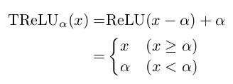
* `alpha` is a learned parameter.
* TReLUs play better with their WN layers than normal ReLUs.
* Reconstruction measure
* To evaluate the quality of the generated images during training, they introduce a new measure.
* The measure is based on a L2-Norm (MSE) between (1) a real image and (2) an image created by the generator that is as similar as possible to the real image.
* They generate (2) by starting `G(z)` with a noise vector `z` that is filled with zeros. The desired output is the real image. They compute a MSE between the generated and real image and backpropagate the result. Then they use the generated gradient to update `z`, while leaving the parameters of `G` unaltered. They repeat this for a defined number of steps.
* Note that the above described method is fairly time-consuming, so they don't do it often.
* Networks
* Their networks are fairly standard.
* Generator: Starts at 1024 filters, goes down to 64 (then 3 for the output). Upsampling via fractionally strided convs.
* Discriminator: Starts at 64 filters, goes to 1024 (then 1 for the output). Downsampling via strided convolutions.
* They test three variations of these networks:
* Vanilla: No normalization. PReLUs in both G and D.
* BN: BN in G and D, but not in the last layers and not in the first layer of D. PReLUs in both G and D.
* WN: Strict weight-normalized layers in G and D, except for the last layers, which are affine weight-normalized layers. TPReLUs (Translated PReLUs) in both G and D.
* Other
* They train with RMSProp and batch size 32.
### Results
* Their WN formulation trains stable, provided the learning rate is set to 0.0002 or lower.
* They argue, that their achieved stability is similar to the one in WGAN.
* BN had significant swings in quality.
* Vanilla collapsed sooner or later.
* Both BN and Vanilla reached an optimal point shortly after the start of the training. After that, the quality of the generated images only worsened.
* Plot of their quality measure:
* 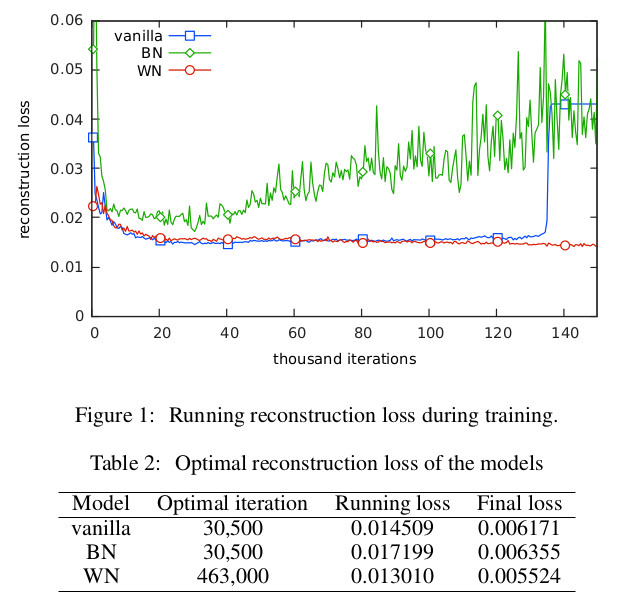
* Their quality measure is based on reconstruction of input images. The below image shows examples for that reconstruction (each person: original image, vanilla reconstruction, BN rec., WN rec.).
* 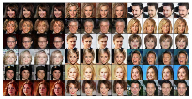
* Examples generated by their WN network:
* 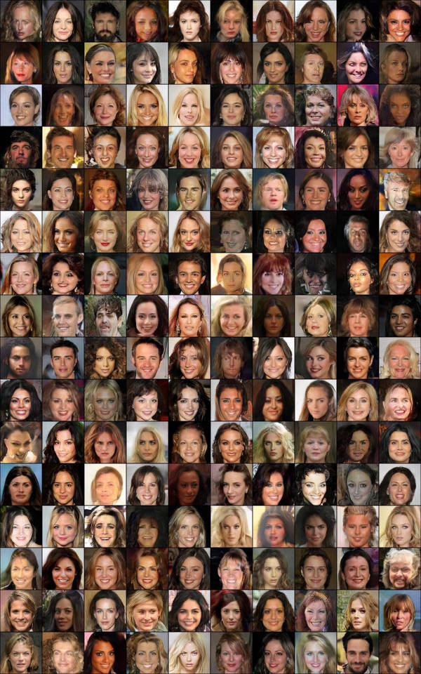
|
MobileNets: Efficient Convolutional Neural Networks for Mobile Vision Applications
Howard, Andrew G. and Zhu, Menglong and Chen, Bo and Kalenichenko, Dmitry and Wang, Weijun and Weyand, Tobias and Andreetto, Marco and Adam, Hartwig
arXiv e-Print archive - 2017 via Local Bibsonomy
Keywords: dblp
Howard, Andrew G. and Zhu, Menglong and Chen, Bo and Kalenichenko, Dmitry and Wang, Weijun and Weyand, Tobias and Andreetto, Marco and Adam, Hartwig
arXiv e-Print archive - 2017 via Local Bibsonomy
Keywords: dblp
|
[link]
* They suggest a factorization of standard 3x3 convolutions that is more efficient.
* They build a model based on that factorization. The model has hyperparameters to choose higher performance or higher accuracy.
### How
* Factorization
* They factorize the standard 3x3 convolution into one depthwise 3x3 convolution, followed by a pointwise convoluton.
* Normal 3x3 convolution:
* Computes per filter and location a weighted average over all filters.
* For kernel height `kH`, width `kW` and number of input filters/planes `Fin`, it requires `kH*kW*Fin` computations per location.
* Depthwise 3x3 convolution:
* Computes per filter and location a weighted average over *one* input filter. E.g. the 13th filter would only computed weighted averages over the 13th input filter/plane and ignore all the other input filters/planes.
* This requires `kH*kW*1` computations per location, i.e. drastically less than a normal convolution.
* Pointwise convolution:
* This is just another name for a normal 1x1 convolution.
* This is placed after a depthwise convolution in order to compensate the fact that every (depthwise) filter only sees a single input plane.
* As the kernel size is `1`, this is rather fast to compute.
* Visualization of normal vs factorized convolution:
* 
* Models
* They use two hyperparameters for their models.
* `alpha`: Multiplier for the width in the range `(0, 1]`. A value of 0.5 means that every layer has half as many filters.
* `roh`: Multiplier for the resolution. In practice this is simply the input image size, having a value of `{224, 192, 160, 128}`.
### Results
* ImageNet
* Compared to VGG16, they achieve 1 percentage point less accuracy, while using only about 4% of VGG's multiply and additions (mult-adds) and while using only about 3% of the parameters.
* Compared to GoogleNet, they achieve about 1 percentage point more accuracy, while using only about 36% of the mult-adds and 61% of the parameters.
* Note that they don't compare to ResNet.
* Results for architecture choices vs. accuracy on ImageNet:
* 
* Relation between mult-adds and accuracy on ImageNet:
* 
* Object Detection
* Their mAP is a bit on COCO when combining MobileNet with SSD (as opposed to using VGG or Inception v2).
* Their mAP is quite a bit worse on COCO when combining MobileNet with Faster R-CNN.
* Reducing the number of filters (`alpha`) influences the results more than reducing the input image resolution (`roh`).
* Making the models shallower influences the results more than making them thinner.
|
Clinical Intervention Prediction and Understanding using Deep Networks
Harini Suresh and Nathan Hunt and Alistair Johnson and Leo Anthony Celi and Peter Szolovits and Marzyeh Ghassemi
arXiv e-Print archive - 2017 via Local arXiv
Keywords: cs.LG
First published: 2017/05/23 (6 years ago)
Abstract: Real-time prediction of clinical interventions remains a challenge within intensive care units (ICUs). This task is complicated by data sources that are noisy, sparse, heterogeneous and outcomes that are imbalanced. In this paper, we integrate data from all available ICU sources (vitals, labs, notes, demographics) and focus on learning rich representations of this data to predict onset and weaning of multiple invasive interventions. In particular, we compare both long short-term memory networks (LSTM) and convolutional neural networks (CNN) for prediction of five intervention tasks: invasive ventilation, non-invasive ventilation, vasopressors, colloid boluses, and crystalloid boluses. Our predictions are done in a forward-facing manner to enable "real-time" performance, and predictions are made with a six hour gap time to support clinically actionable planning. We achieve state-of-the-art results on our predictive tasks using deep architectures. We explore the use of feature occlusion to interpret LSTM models, and compare this to the interpretability gained from examining inputs that maximally activate CNN outputs. We show that our models are able to significantly outperform baselines in intervention prediction, and provide insight into model learning, which is crucial for the adoption of such models in practice.
more
less
Harini Suresh and Nathan Hunt and Alistair Johnson and Leo Anthony Celi and Peter Szolovits and Marzyeh Ghassemi
arXiv e-Print archive - 2017 via Local arXiv
Keywords: cs.LG
First published: 2017/05/23 (6 years ago)
Abstract: Real-time prediction of clinical interventions remains a challenge within intensive care units (ICUs). This task is complicated by data sources that are noisy, sparse, heterogeneous and outcomes that are imbalanced. In this paper, we integrate data from all available ICU sources (vitals, labs, notes, demographics) and focus on learning rich representations of this data to predict onset and weaning of multiple invasive interventions. In particular, we compare both long short-term memory networks (LSTM) and convolutional neural networks (CNN) for prediction of five intervention tasks: invasive ventilation, non-invasive ventilation, vasopressors, colloid boluses, and crystalloid boluses. Our predictions are done in a forward-facing manner to enable "real-time" performance, and predictions are made with a six hour gap time to support clinically actionable planning. We achieve state-of-the-art results on our predictive tasks using deep architectures. We explore the use of feature occlusion to interpret LSTM models, and compare this to the interpretability gained from examining inputs that maximally activate CNN outputs. We show that our models are able to significantly outperform baselines in intervention prediction, and provide insight into model learning, which is crucial for the adoption of such models in practice.
|
[link]
#### Goal: Predict interventions on ICU patients using LSTM and CNN. #### Dataset: MIMIC-III v.1.4 https://mimic.physionet.org/ + Patients over 15 years of age with intensive care stay between 12h and 240h. (Only the first stay is considered for each patient) - 34148 unique records. + 5 static variables. + 29 vital signs and test results. + Clinical notes of patients (presented as time series). #### Feature Engineering: + Topic Modeling of clinical notes: Vector of topics using Latent Dirichlet Allocation (LDA) + Physiological Words: Vital / Laboratory results converted to z-scores - [integer values between -4 and 4] and score is one-hot encoded (each vital / lab is replaced by 9 columns). It is good idea to avoid the imputation of missing values as the physiological word in this case is the all-zero vector. Feature vector: + is the concatenation of the static variables, physiological words for each vital/lab and the topic vector. + 1 feature vector / patient / hour. + 6-hour slice used to predict a 4-hour window after a 6-hour gap. All the features values are normalized between 0 and 1. (static variables are replicated). #### Target Classes: For some of the procedures to be predicted there are 4 classes: + Onset: Y goes from 0 to 1 during the prediction window. + Wean: Y goes from 1 to 0 during the prediction window. + Stay On: Y stays at 1 throughout prediction window. + Stay Off: Y stays at 0 for the entire prediction window. #### Setup of the Experiments: + Dataset Split: 70% training, 10% validation, 20% test. Long Short Term Memory (LSTM) Networks: + Dropout P(keep) = 0.8, L2 regularization. + 2 hidden layers: 512 nodes in each. Convolutional Neural Networks + 3 different temporal granularities (3, 4, 5 hours). 64 filters in each. + Features are treated as channels. 1D temporal convolution. + Dropout between fully connected layers. P (keep) = 0.5. TensorFlow 1.0.1 - Adam optimizer. Minibatches of size 128. Validation set used for early stopping (metric: AUC). #### Results: + Baseline for comparison: L2-regularized Logistic Regression + Metrics: + AUC per class. + AUC macro = Arithmetic mean of AUC per class. + Proposed architectures outperforms baseline. + Physiological words improve performance (especially on high class imbalance scenario). #### Model Interpretability: + LSTM: feature occlusion like analysis. The feature is replaced by uniformly distributed noise between 0 and 1 and variation in AUC is computed. + CNN: analysis of the maximally activating trajectories. #### Positive Aspects: + Relevant work: In the healthcare domain is very important to anticipate events. + Built on top of rich and heterogeneous data: It leverages large amounts of ICU data. + The proposed model is not a complete black-box. Interpretability is crucial if the system is to be adopted in the future. #### Caveats: + Some of the methodology is not clearly explained: + How the split of the dataset was performed? Was it on a patient-level? + When testing the logistic regression baseline it is not clear how the feature vector was built. Was it built by simply flattening the 6-hour chunk? + For the raw data test, it was not mentioned the way the missing values were treated. |

Learning Important Features Through Propagating Activation Differences
Shrikumar, Avanti and Greenside, Peyton and Kundaje, Anshul
International Conference on Machine Learning - 2017 via Local Bibsonomy
Keywords: dblp
Shrikumar, Avanti and Greenside, Peyton and Kundaje, Anshul
International Conference on Machine Learning - 2017 via Local Bibsonomy
Keywords: dblp
|
[link]
### Summary

The motivation of this paper is to make neural network interpretable so that they can be adopted in fields where interpretability is essential (ie: medical field). Thus, this paper present _DeepLIFT_, a method to interpret neural networks by **decomposing** the output prediction given a specific input by backpropagating the _contribution_ of all the neurons to every input features. The _contribution_ of a neuron is determined by comparing the activation of this neuron to a _reference activation_. This _reference activation_ is determined arbitrarily by a domain expert. Moreover, the authors argue that in some case, giving separate consideration to positive and negative contributions can reveal dependencies that are missed by other approaches. The authors show that their approaches can capture some dependencies that a gradient-based method cannot.

### Computing the contribution of a neuron

Given the following notation:
* $t$: Target output neuron
* $t^0$: Reference activation of $t$
* $x_1, x_2, ..., x_n$: Set of neurons
* $\Delta t$: The difference-from-reference of a target
* $\Delta x$: The difference-from-reference of an input
* $C_{\Delta x_i,\Delta t}$: Contributions scores of a neuron

$$\Delta t = t - t^0$$
$$\Delta t = \sum_{i=1}^n C_{\Delta x_i \Delta t}$$

The advantage of the _difference from reference_ against purely gradient method is that the _diference from reference_ avoid all discontinuities as seen in the following figure

https://i.imgur.com/vLZytJT.png

### "Backpropagating" the contribution to the input

To compute the contribution to the input, the authors use a concept similar to the chain rule. Given a _multiplier_ $m_\Delta x _\Delta t$ computed as following:

$$m_{\Delta x \Delta t} = \frac{C_{\Delta x \Delta t}} {\Delta x}$$

Given $z$ the output of a neuron, $y_j$ one neuron in the hidden layer before $z$ and $x_i$ one neuron at the input, before $y_j$. We can compute $m_{\Delta x_i \Delta z}$ as following:

$$m_{\Delta x_i \Delta z}=\sum_j m_{\Delta x_i \Delta y_j} m_{\Delta y_j \Delta z}$$

### Computing the contribution score

The authors argues that it can be beneficial in some case to separate the positive and negative contributions. ie:
$$\Delta _{x_i} = \Delta _{x_i}^+ + \Delta _{x_i}^-$$
$$C_{\Delta _{x_i} \Delta _t} = C_{\Delta _{x_i}^+ \Delta _t} + C_{\Delta _{x_i}^- \Delta _t}$$

The authors propose three similars techniques to compute the contribution score

1. A linear rule where one does not take into consideration the nonlinearity function such that $C_{\Delta _{x_i} \Delta _t} = w_i \Delta _{x_i}$
2. The _rescale rule_ applied to nonlinear function (ie: $y=f(x)$). If $\Delta _y = 0$ or is very close (less than $10^{-7}$), then the authors use the gradient instead of the multiplier.
3. The _Reveal Cancel rule_ is similar than the _rescale rule_, but threat the positive and negative example differently. This allows to capture dependencies (ie: min/AND) that cannot be captured by _rescale rule_ or other method. The difference from reference can be computed as follow:
$$\Delta y^+ = \frac{1}{2}(f(x^0 + \Delta x^+) - f(x^0)) + \frac{1}{2}(f(x^0 + \Delta x^+ + \Delta x^-) - f(x^0+ \Delta x^-)$$
$$\Delta y^- = \frac{1}{2}(f(x^0 + \Delta x^-) - f(x^0)) + \frac{1}{2}(f(x^0 + \Delta x^+ + \Delta x^-) - f(x^0+ \Delta x^+)$$
1 Comments
 |

Representation Learning by Rotating Your Faces
Tran, Luan and Yin, Xi and Liu, Xiaoming
arXiv e-Print archive - 2017 via Local Bibsonomy
Keywords: dblp
Tran, Luan and Yin, Xi and Liu, Xiaoming
arXiv e-Print archive - 2017 via Local Bibsonomy
Keywords: dblp
|
[link]
This paper gets a face image and changes its pose or rotates it (to any desired pose) by passing the target pose as the input to the model. https://i.imgur.com/AGNOag5.png They use a GAN (named DR-GAN) for face rotation. The gan has an encoder and a decoder. The encoder takes the image and gets a high-level feature representation. The decoder gets high-level features, the target pose, and some noise to generate the output image with rotated face. The generated image is then passed to a discriminator where it says whether the image is real or fake. The disc also has two other outputs: 1- it estimates the pose of the generated image, 2) it estimated the identity of the person. no direct loss is applied to the generator, it is trained by the gradient that it gets through discriminator to minimize the three objects: 1- gan loss (to fool disc) 2-pose estimation 3- identity estimation. They use two tricks to improve the model: 1- using the same parameters for encoder of generator (gen-enc) and the discriminator (they observe this helps better identity recognition) 2- passing two images to gen-enc and interpolating between their high-level features (gen-enc output) and then applying two costs on it: 1) gan loss 2) pose loss. These losses are applied through disc, similar to above. The first trick improves gen-enc and second trick improves gen-dec, both help on identification. Their model can also leverage multiple image of the same identity if the dataset provides that to get better latent representation in gen-enc for a given identity. https://i.imgur.com/23Tckqc.png These are some samples on face frontalization: https://i.imgur.com/zmCODXe.png and these are some samples on interpolating different features in latent space: (sub-fig a) interpolating f(x) between the latent space of two images, (sub-fig b) interpolating pose (c), (sub-fig c) interpolating noise: https://i.imgur.com/KlkVyp9.png I find these positive aspects about the paper: 1) face rotation is applied on the images in the wild, 2) It is not required to have paired data. 3) multiple source images of the same identity can be used if provided, 4) identity and pose are used smartly in the discriminator to guide the generator, 5) model can specify the target pose (it is not only face-frontalization). Negative aspects: 1) face has many artifacts, similar to artifacts of some other gan models. 2) The identity is not well-preserved and the faces seem sometime distorted compared to the original person. They show the models performance on identity recognition and face rotation and demonstrate compelling results. |
Squeeze-and-Excitation Networks
Jie Hu and Li Shen and Gang Sun
arXiv e-Print archive - 2017 via Local arXiv
Keywords: cs.CV
First published: 2017/09/05 (6 years ago)
Abstract: Convolutional neural networks are built upon the convolution operation, which extracts informative features by fusing spatial and channel-wise information together within local receptive fields. In order to boost the representational power of a network, much existing work has shown the benefits of enhancing spatial encoding. In this work, we focus on channels and propose a novel architectural unit, which we term the "Squeeze-and-Excitation" (SE) block, that adaptively recalibrates channel-wise feature responses by explicitly modelling interdependencies between channels. We demonstrate that by stacking these blocks together, we can construct SENet architectures that generalise extremely well across challenging datasets. Crucially, we find that SE blocks produce significant performance improvements for existing state-of-the-art deep architectures at slight computational cost. SENets formed the foundation of our ILSVRC 2017 classification submission which won first place and significantly reduced the top-5 error to 2.251%, achieving a 25% relative improvement over the winning entry of 2016.
more
less
Jie Hu and Li Shen and Gang Sun
arXiv e-Print archive - 2017 via Local arXiv
Keywords: cs.CV
First published: 2017/09/05 (6 years ago)
Abstract: Convolutional neural networks are built upon the convolution operation, which extracts informative features by fusing spatial and channel-wise information together within local receptive fields. In order to boost the representational power of a network, much existing work has shown the benefits of enhancing spatial encoding. In this work, we focus on channels and propose a novel architectural unit, which we term the "Squeeze-and-Excitation" (SE) block, that adaptively recalibrates channel-wise feature responses by explicitly modelling interdependencies between channels. We demonstrate that by stacking these blocks together, we can construct SENet architectures that generalise extremely well across challenging datasets. Crucially, we find that SE blocks produce significant performance improvements for existing state-of-the-art deep architectures at slight computational cost. SENets formed the foundation of our ILSVRC 2017 classification submission which won first place and significantly reduced the top-5 error to 2.251%, achieving a 25% relative improvement over the winning entry of 2016.
|
[link]
"The SE module can learn some nonlinear global interactions already known to be useful, such as spatial normalization. The channel wise weights make it somewhat more powerful than divisive normalization as it can learn feature-specific inhibitions (ie: if we see a lot of flower parts, the probability of boat features should be diminished). It also has some similarity to bio inhibitory circuits." By jcannell on reddit Slides: http://image-net.org/challenges/talks_2017/SENet.pdf Summary by the author Jie Hu: Our motivation is to explicitly model the interdependence between feature channels. In addition, we do not intend to introduce a new spatial dimension for the integration of feature channels, but rather a new "feature re-calibration" strategy. Specifically, it is through learning the way to automatically obtain the importance of each feature channel, and then in accordance with this importance to enhance the useful features and inhibit the current task is not useful features. https://i.imgur.com/vXyBg4j.png The above figure is a schematic diagram of our proposed SE module. Given an input $x$, the number of characteristic channels is $c_1$, and the characteristic number of a characteristic channel is $c_2$ by a series of convolution and other general transformations. Unlike traditional CNNs, we then re-calibrate the features we received in the next three operations. The first is the Squeeze operation, we carry out the feature compression along the spatial dimension, and turn each two-dimensional feature channel into a real number. The real number has a global sense of the wild, and the output dimension and the number of input channels Match. It characterizes the global distribution of responses on the feature channel, and makes it possible to obtain a global sense of the field near the input, which is very useful in many tasks. Followed by the Excitation operation, which is a mechanism similar to the door in a circular neural network. The weight is generated for each feature channel by the parameter $w$, where the parameter w is learned to explicitly model the correlation between the feature channels. Reddit thread: https://www.reddit.com/r/MachineLearning/comments/6pt99z/r_squeezeandexcitation_networks_ilsvrc_2017/ |
The Shattered Gradients Problem: If resnets are the answer, then what is the question?
Balduzzi, David and Frean, Marcus and Leary, Lennox and Lewis, J. P. and Ma, Kurt Wan-Duo and McWilliams, Brian
International Conference on Machine Learning - 2017 via Local Bibsonomy
Keywords: dblp
Balduzzi, David and Frean, Marcus and Leary, Lennox and Lewis, J. P. and Ma, Kurt Wan-Duo and McWilliams, Brian
International Conference on Machine Learning - 2017 via Local Bibsonomy
Keywords: dblp
|
[link]
Imagine you make a neural network mapping a scalar to a scalar. After you initialise this network in the traditional way, randomly with some given variance, you could take the gradient of the input with respect to the output for all reasonable values (between about - and 3 because networks typically assume standardised inputs). As the value increases, different rectified linear units in the network will randomly switch on, drawing a random walk in the gradients; another name for which is brown noise.

However, do the same thing for deep networks, and any traditional initialisation you choose, and you'll see the random walk start to look like white noise. One intuition given in the paper is that as different rectifiers in the network switch off and on the input is taking a number of different paths though the network. The number of possible paths grows exponentially with the depth of the network, so as the input varies, the gradients become increasingly chaotic. **The explanations and derivations given in the paper are much better reasoned and thorough, please read those if you are interested**.
Why should we care about this? Because the authors take the recent nonlinearity [CReLU][] (output is concatenation of `relu(x)` and `relu(-x)`) and develop an initialisation that will avoid problems with gradient shattering. The initialisation is just to take your standard initialised weight matrix $\mathbf{W}$ and set the right half to be the negative of the left half ($\mathbf{W}_{\text{left}}$). As long as the input to the layer is also concatenated, the left half will be multiplied by `relu(x)` and the right by `relu(-x)`. Then:
$$
\mathbf{W}.\text{CReLU}(\mathbf{x}) = \begin{cases} \mathbf{W}_{\text{left}}\mathbf{x} & \text{ if } x > 0 \\ \mathbf{W}_{\text{left}}\mathbf{x} & \text{ if } x \leq 0\end{cases}
$$
Doing this allows them to train deep networks without skip connections, and they show results on CIFAR-10 with depths of up to 200 exceeding (slightly) a similar resnet.
[crelu]: https://arxiv.org/abs/1603.05201
|
A Deep Compositional Framework for Human-like Language Acquisition in Virtual Environment
Yu, Haonan and Zhang, Haichao and Xu, Wei
arXiv e-Print archive - 2017 via Local Bibsonomy
Keywords: dblp
Yu, Haonan and Zhang, Haichao and Xu, Wei
arXiv e-Print archive - 2017 via Local Bibsonomy
Keywords: dblp
|
[link]
This paper proposes a framework where an agent learns to navigate a 2D maze-like environment (XWORLD) from (templated) natural language commands, in the process simultaneously learning visual representations, syntax and semantics of language and performing navigation actions. The task is essentially VQA + navigation; at every step the agent either gets a question about the environment or navigation command, and the output is either a navigation action or answer. Key contributions: - Grounding and recognition are tied together to be two versions of the same problem. In grounding, given an image feature map and label (word), the problem is to find regions of the image corresponding to word semantics (attention map); and in recognition, given an image feature map and attention, the problem is to assign a word label. And thus word embeddings (for grounding) and softmax layer weights (for recognition) are tied together. This enables transferring concepts learnt during recognition to navigation. - Further, recognition is modulated by question intent. For e.g. given an attention map that highlights an agent's west, should it be recognized as 'west', 'apple' or 'red' (location, object or attribute)? It depends on what the question asks. Thus, GRU encoding of question produces an embedding mask that modulates recognition. The equivalent when grounding is that word embeddings are passed through fully-connected layers. - Compositionality in language is exploited by performing grounding and recognition by sequentially (softly) attending to parts of a sentence and grounding in image. The resulting attention map is selectively combined with attention from previous timesteps for final decision. ## Weaknesses / Notes Although the environment is super simple, it's a neat framework and it is useful that the target is specified in natural language (unlike prior/concurrent work e.g. Zhu et al., ICRA17). The model gets to see a top-down centred view of the entire environment at all times, which is a little weird. |

A simple neural network module for relational reasoning
Adam Santoro and David Raposo and David G. T. Barrett and Mateusz Malinowski and Razvan Pascanu and Peter Battaglia and Timothy Lillicrap
arXiv e-Print archive - 2017 via Local arXiv
Keywords: cs.CL, cs.LG
First published: 2017/06/05 (6 years ago)
Abstract: Relational reasoning is a central component of generally intelligent behavior, but has proven difficult for neural networks to learn. In this paper we describe how to use Relation Networks (RNs) as a simple plug-and-play module to solve problems that fundamentally hinge on relational reasoning. We tested RN-augmented networks on three tasks: visual question answering using a challenging dataset called CLEVR, on which we achieve state-of-the-art, super-human performance; text-based question answering using the bAbI suite of tasks; and complex reasoning about dynamic physical systems. Then, using a curated dataset called Sort-of-CLEVR we show that powerful convolutional networks do not have a general capacity to solve relational questions, but can gain this capacity when augmented with RNs. Our work shows how a deep learning architecture equipped with an RN module can implicitly discover and learn to reason about entities and their relations.
more
less
Adam Santoro and David Raposo and David G. T. Barrett and Mateusz Malinowski and Razvan Pascanu and Peter Battaglia and Timothy Lillicrap
arXiv e-Print archive - 2017 via Local arXiv
Keywords: cs.CL, cs.LG
First published: 2017/06/05 (6 years ago)
Abstract: Relational reasoning is a central component of generally intelligent behavior, but has proven difficult for neural networks to learn. In this paper we describe how to use Relation Networks (RNs) as a simple plug-and-play module to solve problems that fundamentally hinge on relational reasoning. We tested RN-augmented networks on three tasks: visual question answering using a challenging dataset called CLEVR, on which we achieve state-of-the-art, super-human performance; text-based question answering using the bAbI suite of tasks; and complex reasoning about dynamic physical systems. Then, using a curated dataset called Sort-of-CLEVR we show that powerful convolutional networks do not have a general capacity to solve relational questions, but can gain this capacity when augmented with RNs. Our work shows how a deep learning architecture equipped with an RN module can implicitly discover and learn to reason about entities and their relations.
|
[link]
This paper describes using Relation Networks (RN) for reasoning about relations between objects/entities. RN is a plug-and-play module and although expects object representations as input, the semantics of what an object is need not be specified, so object representations can be convolutional layer feature vectors or entity embeddings from text, or something else. And the feedforward network is free to discover relations between objects (as opposed to being hand-assigned specific relations). - At its core, RN has two parts: - a feedforward network `g` that operates on pairs of object representations, for all possible pairs, all pairwise computations pooled via element-wise addition - a feedforward network `f` that operates on pooled features for downstream task, everything being trained end-to-end - When dealing with pixels (as in CLEVR experiment), individual object representations are spatially distinct convolutional layer features (196 512-d object representations for VGG conv5 say). The other experiment on CLEVR uses explicit factored object state representations with 3D coordinates, shape, material, color, size. - For bAbI, object representations are LSTM encodings of supporting sentences. - For VQA tasks, `g` conditions its processing on question encoding as well, as relations that are relevant for figuring out the answer would be question-dependent. ## Strengths - Very simple idea, clearly explained, performs well. Somewhat shocked that it hasn't been tried before. ## Weaknesses / Notes Fairly simple idea — let a feedforward network operate on all pairs of object representations and figure out relations necessary for downstream task with end-to-end training. And it is fairly general in its design, relations aren't hand-designed and neither are object representations — for RGB images, these are spatially distinct convolutional layer features, for text, these are LSTM encodings of supporting facts, and so on. This module can be dropped in and combined with more sophisticated networks to improve performance at VQA. RNs also offer an alternative design choice to prior works on CLEVR, that have this explicit notion of programs or modules with specialized roles (that need to be pre-defined), as opposed to letting these relations emerge, reducing dependency on hand-designing modules and adding in inductive biases from an architectural point-of-view for the network to reason about relations (earlier end-to-end VQA models didn't have the capacity to figure out relations). |
Towards Diverse and Natural Image Descriptions via a Conditional GAN
Bo Dai and Sanja Fidler and Raquel Urtasun and Dahua Lin
arXiv e-Print archive - 2017 via Local arXiv
Keywords: cs.CV
First published: 2017/03/17 (7 years ago)
Abstract: Despite the substantial progress in recent years, the image captioning techniques are still far from being perfect.Sentences produced by existing methods, e.g. those based on RNNs, are often overly rigid and lacking in variability. This issue is related to a learning principle widely used in practice, that is, to maximize the likelihood of training samples. This principle encourages high resemblance to the "ground-truth" captions while suppressing other reasonable descriptions. Conventional evaluation metrics, e.g. BLEU and METEOR, also favor such restrictive methods. In this paper, we explore an alternative approach, with the aim to improve the naturalness and diversity -- two essential properties of human expression. Specifically, we propose a new framework based on Conditional Generative Adversarial Networks (CGAN), which jointly learns a generator to produce descriptions conditioned on images and an evaluator to assess how well a description fits the visual content. It is noteworthy that training a sequence generator is nontrivial. We overcome the difficulty by Policy Gradient, a strategy stemming from Reinforcement Learning, which allows the generator to receive early feedback along the way. We tested our method on two large datasets, where it performed competitively against real people in our user study and outperformed other methods on various tasks.
more
less
Bo Dai and Sanja Fidler and Raquel Urtasun and Dahua Lin
arXiv e-Print archive - 2017 via Local arXiv
Keywords: cs.CV
First published: 2017/03/17 (7 years ago)
Abstract: Despite the substantial progress in recent years, the image captioning techniques are still far from being perfect.Sentences produced by existing methods, e.g. those based on RNNs, are often overly rigid and lacking in variability. This issue is related to a learning principle widely used in practice, that is, to maximize the likelihood of training samples. This principle encourages high resemblance to the "ground-truth" captions while suppressing other reasonable descriptions. Conventional evaluation metrics, e.g. BLEU and METEOR, also favor such restrictive methods. In this paper, we explore an alternative approach, with the aim to improve the naturalness and diversity -- two essential properties of human expression. Specifically, we propose a new framework based on Conditional Generative Adversarial Networks (CGAN), which jointly learns a generator to produce descriptions conditioned on images and an evaluator to assess how well a description fits the visual content. It is noteworthy that training a sequence generator is nontrivial. We overcome the difficulty by Policy Gradient, a strategy stemming from Reinforcement Learning, which allows the generator to receive early feedback along the way. We tested our method on two large datasets, where it performed competitively against real people in our user study and outperformed other methods on various tasks.
|
[link]
This paper proposes a conditional GAN-based image captioning model.
Given an image, the generator generates a caption, and given an image
and caption, the discriminator/evaluator distinguishes between generated
and real captions. Key ideas:

- Since caption generation involves sequential sampling, which is
non-differentiable, the model is trained with policy gradients, with
the action being the choice of word at every time step, policy being
the distribution over words, and reward the score assigned by the
evaluator to generated caption.

- The evaluator's role assumes a completely generated caption as input
(along with image), which in practice leads to convergence issues. Thus
to accommodate feedback for partial sequences during training, Monte Carlo
rollouts are used, i.e. given a partial generated sequence, n completions
are sampled and run through the evaluator to compute reward.

- The evaluator's objective function consists of three terms
    - image-caption pairs from training data (positive)
    - image and generated captions (negative)
    - image and sampled captions for other images from training data (negative)

- Both the generator and evaluator are pretrained with supervision / MLE, then
fine-tuned with policy gradients. During inference, evaluator score is used as
the beam search objective.

## Strengths

This is neat paper with insightful ideas (Monte Carlo rollouts for assigning
rewards to partial sequences, evaluator score as beam search objective),
and is perhaps the first work on C-GAN-based image captioning.

## Weaknesses / Notes
|
Deep MR to CT Synthesis using Unpaired Data
Jelmer M. Wolterink and Anna M. Dinkla and Mark H. F. Savenije and Peter R. Seevinck and Cornelis A. T. van den Berg and Ivana Isgum
arXiv e-Print archive - 2017 via Local arXiv
Keywords: cs.CV
First published: 2017/08/03 (6 years ago)
Abstract: MR-only radiotherapy treatment planning requires accurate MR-to-CT synthesis. Current deep learning methods for MR-to-CT synthesis depend on pairwise aligned MR and CT training images of the same patient. However, misalignment between paired images could lead to errors in synthesized CT images. To overcome this, we propose to train a generative adversarial network (GAN) with unpaired MR and CT images. A GAN consisting of two synthesis convolutional neural networks (CNNs) and two discriminator CNNs was trained with cycle consistency to transform 2D brain MR image slices into 2D brain CT image slices and vice versa. Brain MR and CT images of 24 patients were analyzed. A quantitative evaluation showed that the model was able to synthesize CT images that closely approximate reference CT images, and was able to outperform a GAN model trained with paired MR and CT images.
more
less
Jelmer M. Wolterink and Anna M. Dinkla and Mark H. F. Savenije and Peter R. Seevinck and Cornelis A. T. van den Berg and Ivana Isgum
arXiv e-Print archive - 2017 via Local arXiv
Keywords: cs.CV
First published: 2017/08/03 (6 years ago)
Abstract: MR-only radiotherapy treatment planning requires accurate MR-to-CT synthesis. Current deep learning methods for MR-to-CT synthesis depend on pairwise aligned MR and CT training images of the same patient. However, misalignment between paired images could lead to errors in synthesized CT images. To overcome this, we propose to train a generative adversarial network (GAN) with unpaired MR and CT images. A GAN consisting of two synthesis convolutional neural networks (CNNs) and two discriminator CNNs was trained with cycle consistency to transform 2D brain MR image slices into 2D brain CT image slices and vice versa. Brain MR and CT images of 24 patients were analyzed. A quantitative evaluation showed that the model was able to synthesize CT images that closely approximate reference CT images, and was able to outperform a GAN model trained with paired MR and CT images.
|
[link]
https://i.imgur.com/vxBhb7B.png Problem ------------ Convert MR scans to CT scans. General Approach ---------- CycleGAN Dataseet ----------- Unpaired brain CT:MR images. The dataset contains both CT and MR scans of same patient taken on the same day. The volumes are aligned using mutual information and contain some local minor misalignments. Method -------- Train the following models: 1. Syn_ct: CNN: MR -> CT 2. Syn_mr: CNN: CT -> MR 3. Dis_ct: classify real and synthetic CT images (result of Syn_ct) 4. Dis_mr: classify real and synthetic MR images. Syn_mr(Syn_ct(MR Image))) or Syn_mr(CT image) https://i.imgur.com/GqVaskb.png |
Learning Hierarchical Features from Generative Models
Zhao, Shengjia and Song, Jiaming and Ermon, Stefano
arXiv e-Print archive - 2017 via Local Bibsonomy
Keywords: dblp
Zhao, Shengjia and Song, Jiaming and Ermon, Stefano
arXiv e-Print archive - 2017 via Local Bibsonomy
Keywords: dblp
|
[link]
A Critical Paper Review by Alex Lamb: https://www.youtube.com/watch?v=_seX4kZSr_8 |
What Actions are Needed for Understanding Human Actions in Videos?
Gunnar A. Sigurdsson and Olga Russakovsky and Abhinav Gupta
arXiv e-Print archive - 2017 via Local arXiv
Keywords: cs.CV
First published: 2017/08/09 (6 years ago)
Abstract: What is the right way to reason about human activities? What directions forward are most promising? In this work, we analyze the current state of human activity understanding in videos. The goal of this paper is to examine datasets, evaluation metrics, algorithms, and potential future directions. We look at the qualitative attributes that define activities such as pose variability, brevity, and density. The experiments consider multiple state-of-the-art algorithms and multiple datasets. The results demonstrate that while there is inherent ambiguity in the temporal extent of activities, current datasets still permit effective benchmarking. We discover that fine-grained understanding of objects and pose when combined with temporal reasoning is likely to yield substantial improvements in algorithmic accuracy. We present the many kinds of information that will be needed to achieve substantial gains in activity understanding: objects, verbs, intent, and sequential reasoning. The software and additional information will be made available to provide other researchers detailed diagnostics to understand their own algorithms.
more
less
Gunnar A. Sigurdsson and Olga Russakovsky and Abhinav Gupta
arXiv e-Print archive - 2017 via Local arXiv
Keywords: cs.CV
First published: 2017/08/09 (6 years ago)
Abstract: What is the right way to reason about human activities? What directions forward are most promising? In this work, we analyze the current state of human activity understanding in videos. The goal of this paper is to examine datasets, evaluation metrics, algorithms, and potential future directions. We look at the qualitative attributes that define activities such as pose variability, brevity, and density. The experiments consider multiple state-of-the-art algorithms and multiple datasets. The results demonstrate that while there is inherent ambiguity in the temporal extent of activities, current datasets still permit effective benchmarking. We discover that fine-grained understanding of objects and pose when combined with temporal reasoning is likely to yield substantial improvements in algorithmic accuracy. We present the many kinds of information that will be needed to achieve substantial gains in activity understanding: objects, verbs, intent, and sequential reasoning. The software and additional information will be made available to provide other researchers detailed diagnostics to understand their own algorithms.
|
[link]
In this race for getting that extra few % improvement for a '*brand-new'* paper, this paper brings a fresh air by posing some very pertinent questions supported by rigorous experimental analysis. Its an ICCV 2017 paper. The paper talks about understanding activities in videos – both from activity classification and detection perspective. In doing so, the authors examined several datasets, evaluation metrics, algorithms, and pointed to possible future directions worthy of exploring. The default choice in terms of the dataset is Charades. Other than this, multiTHUMOS, THUMOS and ActivityNet are used as and when required. The activity classification/detection algorithms analyzed, are two-stream, improved dense trajectories (IDT), LSTM on VGG, actionVLAD and temporalfields.

The paper starts with the very definition of action. To quote *"When we talk about activities, we are referring to anything a person is doing, regardless of whether the person is intentionally and actively altering the environment, or simply sitting still".* This is a complementary perspective than what the community has perceived as action so far - *"Intentional bodily motion of biological agents"* [1]. The paper generalizes this notion and advocates that bodily motion is not indispensable to define actionness (*e.g.*, 'watching the tv', 'Lying on a couch' hardly consist of a bodily motion). Analysis of motion’s role in understanding activity has played a major role later in the paper. Let’s see some of the major questions that the authors explored in this paper.

1. "Only verbs" can make actions ambiguous. To quote, - "Verbs such as 'drinking' and 'running' are unique on their own, but verbs such as 'take' and 'put' are ambiguous unless nouns and even prepositions are included: 'take medication', 'take shoes', take off shoes'". The experiments involving both human (sec 3.1) and activity algorithms (sec 4.1) shows that given the verb less confusion arises when the object is mentioned ('holding a cup' vs 'holding a broom'), but given the object, confusion is more among different verbs ('holding a cup' vs 'drinking from a cup'). All the current algorithms are shown to have significant confusion among similar action categories, both in terms of verbs and objects. In fact, for a given category, the more categories share the object or verb, the worse is the accuracy.
2. The next study, to me, is the most important one. It’s about the long-standing concern of whether activities have clear and universal boundaries. The human study shows that, in fact, it is ambiguous. Average human agreement with ground truth is only 72.5% IOU for Charades and 58.7% IOU for MultiTHUMOS. In a natural course of action, the authors wanted to see if this ambiguity is affecting the evaluation performance of the algorithms. For this purpose, they relaxed the ground truth boundary to be more flexible (sec 3.2) and then evaluated the performance of the algorithms. The surprising fact is that this relaxation did not improve the performance much. The authors opined that despite boundary ambiguity current datasets allow current algorithms to understand and learn from the temporal extent of activities. I must say, I did not expect that ambiguity in temporal boundary will have this insignificant effect on the localization performances. In addition to the conclusion as drawn by the authors, this can be caused by another issue. The (bad) effect of other things are so large that the correction due to boundary ambiguity can't change the performance much. What I mean is - it may not be that the datasets are sufficient but the algorithms are suffering from other flaws much more than they are suffering from the boundary ambiguity.
3. Another important question that the authors dealt with is – how does the amount of labeled training data affect the performance. The broad finding goes with the common knowledge of - "more data means better performance". However, there are a plethora of finer equally important insights that the authors pointed out. The amount of data does not affect all categories equally, especially for a dataset with long-tailed distribution of classes. Smaller categories are more affected. In addition, activities with more similar categories (that share the same object/verb) also get affected much more than their counter parts. The authors end the subsection (sec 4.2) with an observation that improvement can be made by designing algorithms that are better able to make use of the wealth of data in small categories than in large ones.
4. The authors did a thorough analysis of the role of temporal reasoning (motion, continuity, and temporal context) for activity understanding. The very first finding is that current methods are doing better for longer activities than shorter ones. Another common notion (naive temporal smoothing of the predictions helps improve localization and classification) is also verified.
5. An action is almost invariably related to persons. So, the authors tried to see if person based reasoning helps. For that, they experimented with removing the person from the scene, keeping nothing but the person etc. They also examined how diverse are the datasets in terms of human pose and if injecting human pose information helps the current approaches. The conclusion was that person based reasoning helps and the nature of the videos require the activity understanding approaches to harness pose information for improved performance.
6. Finally, the authors try to see what aspects help most if that aspect is solved perfectly with an oracle. The oracles include perfect object detection, perfect verb identification and so on.  It varies for datasets to some extent but, in general, the finding was that all the oracles help, some more some less.

I think this is a much-needed work that would help the community to ponder over different avenues of activity understanding in videos to design better systems.

[1]. Wei Chen, Caiming Xiong, Ran Xu, Jason J. Corso, Actionness Ranking with Lattice Conditional Ordinal Random Fields, CVPR 2014.
|

On orthogonality and learning recurrent networks with long term dependencies
Eugene Vorontsov and Chiheb Trabelsi and Samuel Kadoury and Chris Pal
arXiv e-Print archive - 2017 via Local arXiv
Keywords: cs.LG, cs.NE
First published: 2017/01/31 (7 years ago)
Abstract: It is well known that it is challenging to train deep neural networks and recurrent neural networks for tasks that exhibit long term dependencies. The vanishing or exploding gradient problem is a well known issue associated with these challenges. One approach to addressing vanishing and exploding gradients is to use either soft or hard constraints on weight matrices so as to encourage or enforce orthogonality. Orthogonal matrices preserve gradient norm during backpropagation and can therefore be a desirable property; however, we find that hard constraints on orthogonality can negatively affect the speed of convergence and model performance. This paper explores the issues of optimization convergence, speed and gradient stability using a variety of different methods for encouraging or enforcing orthogonality. In particular we propose a weight matrix factorization and parameterization strategy through which we can bound matrix norms and therein control the degree of expansivity induced during backpropagation.
more
less
Eugene Vorontsov and Chiheb Trabelsi and Samuel Kadoury and Chris Pal
arXiv e-Print archive - 2017 via Local arXiv
Keywords: cs.LG, cs.NE
First published: 2017/01/31 (7 years ago)
Abstract: It is well known that it is challenging to train deep neural networks and recurrent neural networks for tasks that exhibit long term dependencies. The vanishing or exploding gradient problem is a well known issue associated with these challenges. One approach to addressing vanishing and exploding gradients is to use either soft or hard constraints on weight matrices so as to encourage or enforce orthogonality. Orthogonal matrices preserve gradient norm during backpropagation and can therefore be a desirable property; however, we find that hard constraints on orthogonality can negatively affect the speed of convergence and model performance. This paper explores the issues of optimization convergence, speed and gradient stability using a variety of different methods for encouraging or enforcing orthogonality. In particular we propose a weight matrix factorization and parameterization strategy through which we can bound matrix norms and therein control the degree of expansivity induced during backpropagation.
|
[link]
Here is a video overview:
https://www.youtube.com/watch?v=t-fow6GJepQ

Here is an image of the poster:
https://i.imgur.com/Ti9btj9.png
1 Comments
 |
Lexical Features in Coreference Resolution: To be Used With Caution
Nafise Sadat Moosavi and Michael Strube
Association for Computational Linguistics - 2017 via Local CrossRef
Keywords:
Nafise Sadat Moosavi and Michael Strube
Association for Computational Linguistics - 2017 via Local CrossRef
Keywords:
|
[link]
(Reposting under ACL 2017 version)

Kind of a response/deeper dive into the durret/klein "easy victories" paper. Suggests that a) lexical features they used ("easy victories") are very prone to overfitting. They first show that several state of the art systems that use lexical features, trained on CoNLL data, perform poorly on wikiref, which was annotated using the same guidelines. Meanwhile the stanford sieve system performs about the same on both.
Then they show that a high percentage of gold standard linked headwords in the test set have been seen in the training set, and that a much lower percentage of errors are in the training set, implying that lexical features just allow you to memorize what kinds of things can be linked.
They suggest development of robust features, including using embeddings as lexical features, using lexical representations only for context, and on the evaluation side, using test sets that are different domains than the training set.
|

Unimodal Probability Distributions for Deep Ordinal Classification
Beckham, Christopher and Pal, Christopher J.
International Conference on Machine Learning - 2017 via Local Bibsonomy
Keywords: dblp
Beckham, Christopher and Pal, Christopher J.
International Conference on Machine Learning - 2017 via Local Bibsonomy
Keywords: dblp
|
[link]
Short overview from ICML: https://youtube.com/watch?v=GMG5bFciuIA Long overview from ICML: https://youtu.be/o6dtDuldsEo |
Gradient Episodic Memory for Continuum Learning
Lopez-Paz, David and Ranzato, Marc'Aurelio
arXiv e-Print archive - 2017 via Local Bibsonomy
Keywords: dblp
Lopez-Paz, David and Ranzato, Marc'Aurelio
arXiv e-Print archive - 2017 via Local Bibsonomy
Keywords: dblp
|
[link]
#### About APAD ####
_This summer I've been Interning at an AI lab at BCM, working under
Ankit Patel in his incredible Neuroscience-meets-Deep-Learning group.
This field is moving faster than anything else out there. Keeping intro short,
so full post + inline pictures are on my [blog](http://rayraycano.github.io/data%20science/tech/2017/07/31/A-Paper-a-Day-GEM.html)_

## Basics ##
* __Paper__: [Gradient Episodic Memory for Continuum Learning][GED]
* __Authors__: David Lopez-Paz, Marc'Aurelio Ranzato
* __Organizaitons__: Facebook AI Research (FAIR)
* __Topic__: Coninuum Learning
* __In One Senetence__: _Paz and Ranzato define sorely needed metrics to the
subfield of Continual Learning while developing a gradient-inspired update rule
that avoids catastrophic forgetting_

### Background ###

Paz and Ranzato's continuum learning targets a more general problem of
_catastrophic forgetting_, which the authors describe as "the poor ability of models to
quickly solve new problems, without forgetting previously acquired knowledge."
Recently this has been a hot topic in AI recently, as a flurry of
papers in early summer were released discussing this topic ([Elastic Weight Consolidation][EWC],
[PathNet][PathNet], [iCaRL][iCARL], [Sluice Network][Sluice Network], [Intelligent Synapses][Intelligent Synapses]).
Avoiding catastrophic forgetting and achieving nontrivial _backwards transfer_ (BT) and _forward transfer_ (FT) are major goals for
continual learning models, and in addition, general AI.

__Analogy Alert!__ _As Ankit explained to me originally:
If you know how to play tennis, your experience
*should* aid your ability to pick up ping pong (FT).
In addition, when you return to tennis, your aptitude
in tennis shouldn't decrease (some atheletes argue that they get better
at their primary sport because they've played secondary sports, i.e. BT)._

## Paper Accomplishments ##

1. Of the 5 papers mentioned above, 0 of them formally define metrics for a
continual learner.
2. The gradient-aligning update rule is quite clever and pretty cool.

### The Metrics ###
First, let's take a look at their formal definitions for FT and BT.
They're displayed below. The notation is a bit confusing, so I've done my
 best to parse it.

[Backward And Forward Transfer LaTeX](https://www.dropbox.com/s/qrj6sxkfruj42uk/Screen%20Shot%202017-07-31%20at%204.56.05%20PM.png?dl=1)

T is the total number of tasks, enumerated from 1 to T. The bi vector is the random initialization for each task. I've omitted accuracy from this discussion because it seem too novel in the context of this paper

* Assume a fixed sequence of tasks (Numbered 1 through T)
* Forward transfer is the average accuracy of some task, task _i_, after each
task in the sequence preceding _i_ is completed.
    * Record the score for task _i_ upon random initialization
    * Learn task 1, record your score for task _i_. Learn task 2, record your
     score for task _i_, etc., up until task _i-1_.
    * Subtract from their score upon initialization and average these scores.
* Backwards Transfer is the average accuracy change for task _i_ after each
task afterwards has been completed
    * Record the score for task _i_ after learning it
    * Learn task _i+1_. Now record the score for task _i_. Learn task _i+2_. Record the
    score for task _i_, etc.
    * For each score of task _i_ that recorded after completeing _i_, subtract from the first
    score for task _i_. Average these Scores


#### Gripes about the Metrics ####
In my opinion, these metrics don't generalize well. Continuum Learning (which I presume
is less general than _Continual_ Learning) specifies a sequence of tasks,
 meaning it is sensitive to the order of tasks. In their experiments section,
 they use tasks that theoretically don't depend on the order in which they're learned, so in the
 scheme of their paper this point is moot. However, Continual Learning in general
has no specification on order. Other papers concerning this topic have not discussed
task curriculums at all, while this paper glosses over it.

__A metric I prefer: randomly sample from a pool of tasks
_n_ times. Learn these _n_ tasks in an arbitrary order. Lastly, evaluate accuracy on _i_ (for forward transfer).__
(This can be done over multiple trials to get a robust average)

### Gradient-Aligned Updates ###

For those new to Machine Learning, much of Deep Learning is powered by the
[__backpropagation algorithm__][backprop]. This algorithm calculates an update that
will improve the accuracy for the problem based on an error metric. It does this by calculating what's
called a gradient.

__Analogy Alert!__ : _You shoot a dart at a board. You shot low by some distance __d__.
You correct your mechanics, backwards reasoning from the missed distance, to your
release point, and from there perhaps your throwing velocity.
You can think of these corrections as the gradient, and the linked modification of
all the preceding components as an implementation
of the [chain rule][chainrule]. Disclaimer:
 There is no evidence that the brain implements backpropagation_

So what does Gradient Episodic Memory (GEM) do exactly? Let's start with the Memory
part and go from there

* _Memory_: Recall those sequence of tasks we mentioned earlier? Well for each of those
tasks, let's make sure we don't forget them. We'll keep a portion of them in memory.

* _Episodic_: Let's replay these memories to make sure we're not damaging our accuracy
on these tasks when we learn new ones. By playing them over again, we're basically going through an episode

* _Gradient_: When we look at the episode again, let's make sure the gradient doesn't
go the wrong way. What this means is: let's not unlearn what we learned on the
previous task.

### So How is it Done? ###

[Gradient Update Equation][Gradient Update Equation]

g is the gradient for the current task, while gk is the gradient for each previous task, calculated over the episodes in memory (Mk). The big < > notation is a dot product operator

Dot Products! In order for a gradient update to take place, they compute the dot product
of the current learning task with all the previous tasks in memory. The update is allowed
to take place if the gradient is greater than or equal to 0 for all the episodes. This translates
into constraining your update for one task to not conflict with an update for the previous task.

What if the gradient is going the wrong way? Paz and Ronzato take this gradient update
and project it to the closest possible vector that doesn't go the wrong way
(The proof is in the pudding, eqn. 8 - 13 in the paper. It formulates the optimization as a projection
on to a cone).

[Gradient Update Projection Example][Gradient Update Projection Example]

 Above shows the graphical representation of the gradient update conditions, with the blue
    line being the update for the first task, while the red line is the gradient update for the current task. The right side
    shows an approximation of the optimized projection for the gradient when the dot product is negative.

### Does it work? ###
Yes. Well, kind of.

The focus of this paper was to minimize Backwards Loss (aka
maximize Backwards Transfer). In this sense, they appear to succeed. However,
the small improvements lack error bars, making an unconvincing case (#DLNeedsErrorBars).
Forward Transfer is negligible on all but one experiment (there were three total).

[Results from Paper]

The plots above show performance. The right hand side demonstrates
the accuracy on the first task as the consequent tasks are learned, which each different
colored bar indicating a start to learning for a new task.

#### Knitpicking ####

* The experiments compare against Elastic Weight Consolidation (EWC). However,
EWC was tested and optimized for Reinforcement Learning and Atari Games. I wonder
if an earnest job of optimizing EWC for the tasks at hand was done.

* There is still no metric for parameter conservation as a result of continual/shared learning.
A curve showing the change in accuracy across a set of tasks while increasing
the size of the overall network would be nice. It would be interesting to compare
all the papers on this metric. You could also evaluate the similarity of tasks
(or how well a network learns similarities in tasks) through this method.

### Summary ###
Cool Method.  Nice Paper. Less than satisfying results. But in general a
solid step forward for continual learning/overcoming catastrophic
forgetting.


[EWC]: https://arxiv.org/pdf/1612.00796.pdf
[PathNet]: https://arxiv.org/pdf/1701.08734.pdf
[iCARL]: https://arxiv.org/pdf/1611.07725.pdf
[Sluice Network]: https://arxiv.org/pdf/1705.08142.pdf
[Intelligent Synapses]: https://openreview.net/pdf?id=rJzabxSFg
[Metrics]: https://www.dropbox.com/s/qrj6sxkfruj42uk/Screen%20Shot%202017-07-31%20at%204.56.05%20PM.png?dl=0
[Gradient]: https://www.dropbox.com/s/jye3b3mco5fs277/Screen%20Shot%202017-07-31%20at%204.55.52%20PM.png?dl=0
[Results]: https://www.dropbox.com/s/qvr95xydhtlnijw/Screen%20Shot%202017-07-31%20at%204.55.41%20PM.png?dl=0
[GED]: https://arxiv.org/pdf/1706.08840.pdf
[backprop]:https://en.wikipedia.org/wiki/Backpropagation
[chainrule]:https://en.wikipedia.org/wiki/Chain_rule
[Gradient Update Equation]:https://www.dropbox.com/s/jye3b3mco5fs277/Screen%20Shot%202017-07-31%20at%204.55.52%20PM.png?dl=1
[Gradient Update Projection Example]: https://www.dropbox.com/s/jkdkk8bmz6btl77/Screen%20Shot%202017-07-31%20at%207.36.14%20PM.png?dl=1 "Projection Update"
[Results from Paper]:https://www.dropbox.com/s/qvr95xydhtlnijw/Screen%20Shot%202017-07-31%20at%204.55.41%20PM.png?dl=1
|

Auto-Conditioned LSTM Network for Extended Complex Human Motion Synthesis
Zimo Li and Yi Zhou and Shuangjiu Xiao and Chong He and Hao Li
arXiv e-Print archive - 2017 via Local arXiv
Keywords: cs.LG
First published: 2017/07/17 (6 years ago)
Abstract: We present a real-time method for synthesizing highly complex human motions using a novel LSTM network training regime we call the auto-conditioned LSTM (acLSTM). Recently, researchers have attempted to synthesize new motion by using autoregressive techniques, but existing methods tend to freeze or diverge after a couple of seconds due to an accumulation of errors that are fed back into the network. Furthermore, such methods have only been shown to be reliable for relatively simple human motions, such as walking or running. In contrast, our approach can synthesize arbitrary motions with highly complex styles, including dances or martial arts in addition to locomotion. The acLSTM is able to accomplish this by explicitly accommodating for autoregressive noise accumulation during training. Furthermore, the structure of the acLSTM is modular and compatible with any other recurrent network architecture, and is usable for tasks other than motion. Our work is the first to our knowledge that demonstrates the ability to generate over 18,000 continuous frames (300 seconds) of new complex human motion w.r.t. different styles.
more
less
Zimo Li and Yi Zhou and Shuangjiu Xiao and Chong He and Hao Li
arXiv e-Print archive - 2017 via Local arXiv
Keywords: cs.LG
First published: 2017/07/17 (6 years ago)
Abstract: We present a real-time method for synthesizing highly complex human motions using a novel LSTM network training regime we call the auto-conditioned LSTM (acLSTM). Recently, researchers have attempted to synthesize new motion by using autoregressive techniques, but existing methods tend to freeze or diverge after a couple of seconds due to an accumulation of errors that are fed back into the network. Furthermore, such methods have only been shown to be reliable for relatively simple human motions, such as walking or running. In contrast, our approach can synthesize arbitrary motions with highly complex styles, including dances or martial arts in addition to locomotion. The acLSTM is able to accomplish this by explicitly accommodating for autoregressive noise accumulation during training. Furthermore, the structure of the acLSTM is modular and compatible with any other recurrent network architecture, and is usable for tasks other than motion. Our work is the first to our knowledge that demonstrates the ability to generate over 18,000 continuous frames (300 seconds) of new complex human motion w.r.t. different styles.
|
[link]
Problem ---------- Motion prediction Dataset ---------- CMU Approach -------------- auto-conditioned LSTM - an LSTM network that uses only fraction of the input timestamps, but all of the outputs (a little bit similar to keyframes). https://image.ibb.co/nimSs5/acLSTM.png Video -------- https://www.youtube.com/watch?v=AWlpNeOzMig |
Sentence Simplification with Deep Reinforcement Learning
Zhang, Xingxing and Lapata, Mirella
arXiv e-Print archive - 2017 via Local Bibsonomy
Keywords: dblp
Zhang, Xingxing and Lapata, Mirella
arXiv e-Print archive - 2017 via Local Bibsonomy
Keywords: dblp
|
[link]
* Output can contain several sentences, that are considered as a single long sequence.
* Seq2Seq+attention:
  * Oddly they use the formula used by Bahdanau attention weights to combine the weighted attention $c_t$ with the decoder output $h_t^T =  W_0 \tanh \left( U_h h_t^T + W_h c_t \right) $ while the attention weights are computed with softmax over dot product between encoder and decoder outputs $h_t^T \cdot h_i^S$
  * Glove 300
  * 2 layer LSTM 256
* RL model
  * Reward=Simplicity+Relevance+Fluency = $\lambda^s r^S + \lambda^R r^R + \lambda^F r^F$
    * $r^S = \beta \text{SARI}(X,\hat{Y},Y) + (1-\beta) \text{SARI}(X,Y,\hat{Y})$
    * $r^R$ cosine of output of RNN auto encoder run on input and a separate auto encoder run on output
    * $r^F$ perplexity of LM trained on output
  * Learning exactly as in [MIXER](https://arxiv.org/abs/1511.06732)
* Lexical Simplification model: they train a second model $P_{LS}$ which uses pre-trained attention weights and then use the weighted output of an encoder LSTM as the input to a softmax
|

The Pose Knows: Video Forecasting by Generating Pose Futures
Walker, Jacob and Marino, Kenneth and Gupta, Abhinav and Hebert, Martial
arXiv e-Print archive - 2017 via Local Bibsonomy
Keywords: dblp
Walker, Jacob and Marino, Kenneth and Gupta, Abhinav and Hebert, Martial
arXiv e-Print archive - 2017 via Local Bibsonomy
Keywords: dblp
|
[link]
Problem --------- Video prediction with human objects Contribution -------------- Instead of the common approach of predicting directly in pixel-space, use explicit knowledge of human motion space to predict the future of the video. Approach -------------- 1. VAE to model the possible future movements of humans in the pose space 2. Conditional GAN - use pose information for to predict video in pixel space. https://image.ibb.co/b1omVF/The_pose_knows.png |
Forecasting Human Dynamics from Static Images
Chao, Yu-Wei and Yang, Jimei and Price, Brian L. and Cohen, Scott and Deng, Jia
arXiv e-Print archive - 2017 via Local Bibsonomy
Keywords: dblp
Chao, Yu-Wei and Yang, Jimei and Price, Brian L. and Cohen, Scott and Deng, Jia
arXiv e-Print archive - 2017 via Local Bibsonomy
Keywords: dblp
|
[link]
Problem ------------- Predict human motion from static image http://www-personal.umich.edu/~ywchao/pictures/cvpr2017.png Approach ---------- 1. 2d pose sequence generator 2. convert 2d pose to 3d skeleton https://image.ibb.co/eeBRxv/3D_PFNet.png https://image.ibb.co/kERaVQ/Forecasting_Human_Dynamics_from_Static_Images_architecture.png 3 Step training strategy ------------------------- 1. Train human 2d pose extractor using annotated video with 2d joint positions 2. 3d skeleton extractor: project mocap data to 2d and use as ground truth for training the 2d->3d skeleton converter 3. Full network training Datasets ----------- 1. Penn Action - Annotated human pose in sports image sequences: bench_press, jumping_jacks, pull_ups... 2. MPII - human action videos with annotated single frame 3. Human3.6M - video, depth and mocap. action include: sitting, purchasing, waiting Evaluation ------------- On the following tasks: 1. 2D pose forecasting 2. 3D pose recovery |
Skeleton-aided Articulated Motion Generation
Yichao Yan and Jingwei Xu and Bingbing Ni and Xiaokang Yang
arXiv e-Print archive - 2017 via Local arXiv
Keywords: cs.CV
First published: 2017/07/04 (6 years ago)
Abstract: This work make the first attempt to generate articulated human motion sequence from a single image. On the one hand, we utilize paired inputs including human skeleton information as motion embedding and a single human image as appearance reference, to generate novel motion frames, based on the conditional GAN infrastructure. On the other hand, a triplet loss is employed to pursue appearance-smoothness between consecutive frames. As the proposed framework is capable of jointly exploiting the image appearance space and articulated/kinematic motion space, it generates realistic articulated motion sequence, in contrast to most previous video generation methods which yield blurred motion effects. We test our model on two human action datasets including KTH and Human3.6M, and the proposed framework generates very promising results on both datasets.
more
less
Yichao Yan and Jingwei Xu and Bingbing Ni and Xiaokang Yang
arXiv e-Print archive - 2017 via Local arXiv
Keywords: cs.CV
First published: 2017/07/04 (6 years ago)
Abstract: This work make the first attempt to generate articulated human motion sequence from a single image. On the one hand, we utilize paired inputs including human skeleton information as motion embedding and a single human image as appearance reference, to generate novel motion frames, based on the conditional GAN infrastructure. On the other hand, a triplet loss is employed to pursue appearance-smoothness between consecutive frames. As the proposed framework is capable of jointly exploiting the image appearance space and articulated/kinematic motion space, it generates realistic articulated motion sequence, in contrast to most previous video generation methods which yield blurred motion effects. We test our model on two human action datasets including KTH and Human3.6M, and the proposed framework generates very promising results on both datasets.
|
[link]
Problem --------------- Video generation of human motion given: 1. Single appearance reference image 2. Skeleton motion sequence Datasets ----------- * KTH - grayscale human actions * Human3.6M - color multiview human actions Approach --------------- Conditional GANs. The authors try both Stack GAN and Siamese GAN. The later provides better result. https://preview.ibb.co/ighxQQ/Skeleton_aided_Articulated_Motion_Generation.png Questions ---------------- Isn't using a full sequence of human skeleton motion considered more then a "hint"? |
Learning to Learn: Meta-Critic Networks for Sample Efficient Learning
Sung, Flood and Zhang, Li and Xiang, Tao and Hospedales, Timothy M. and Yang, Yongxin
arXiv e-Print archive - 2017 via Local Bibsonomy
Keywords: dblp
Sung, Flood and Zhang, Li and Xiang, Tao and Hospedales, Timothy M. and Yang, Yongxin
arXiv e-Print archive - 2017 via Local Bibsonomy
Keywords: dblp
|
[link]
At the core of an actor-critic algorithm is an idea of approximating an objective function $Q(s, a)$ (or Q function) with a trainable function $Q_\theta$ called a critic. An actor $\pi_\phi$ is then trained to maximize $Q_\theta$ instead of the original $Q$. Often, a pair of $Q_\theta$ and $\pi_\phi$ are trained separately for each task $\mathcal{T}$. In this paper, the authors cleverly propose to share a single critic $Q_\theta$ across multiple tasks $\mathcal{T}_1, \ldots, \mathcal{T}_L$ by parametrizing it to be dependent on a task. That is, $Q_\theta(s, a, z)$, where $z$ is a task vector.

For simplicity, consider a supervised learning task (as in Sec. 3.2), where $Q^t$ is an objective function for the $t$-th task and takes as input a training example pair $(x, y)$. A single critic $Q_\theta$ is then trained to approximate $L$-many such objective functions, i.e., $\arg\min_{\theta} \sum_{t=1}^L \sum_{(x,y)} (Q^t(x,y) - Q_\theta(x,y,z^t))^2$. The task vector $z^t$ is obtained by a task encoder (TAEN) which takes as input a minibatch of training examples of the $t$-th task and outputs the task vector. The TAEN is trained together with the $Q_\theta$, and all the $L$ actors $\pi^t$.

Once the critic (or meta-critic, as referred to by the authors) is trained, a new actor $\pi_\phi^{L+1}$ can be trained based on a small set of training examples in the following steps. First, the small set of training examples are used to compute a new task vector $z^{L+1}$. Second, a new critic is computed: $Q_\theta(\cdot,\cdot,z^{L+1})$. Third, the new actor is trained to maximize the new critic.

One big lesson I learned from this paper is that there are different ways to approach meta-learning. In the context of iterative learning of neural nets, I've only thought of meta-learning as learning to approximate an update direction as from https://arxiv.org/abs/1606.04474, i.e., $\phi \leftarrow \phi + g_\theta(\phi, x, y)$. This paper however suggests that you can instead learn an objective function, i.e., $\phi \leftarrow \phi + \eta \nabla_{\phi} Q_\theta(x, \pi_{\phi}(x), z(D))$, where $z(D)$ is a task vector obtained from new data $D$.
This is interesting, as it maximally reuses any existing technique from gradient-based learning and frees the meta-learner from having to re-learn them again.
|

Bayesian Compression for Deep Learning
Christos Louizos and Karen Ullrich and Max Welling
arXiv e-Print archive - 2017 via Local arXiv
Keywords: stat.ML, cs.LG
First published: 2017/05/24 (6 years ago)
Abstract: Compression and computational efficiency in deep learning have become a problem of great significance. In this work, we argue that the most principled and effective way to attack this problem is by taking a Bayesian point of view, where through sparsity inducing priors we prune large parts of the network. We introduce two novelties in this paper: 1) we use hierarchical priors to prune nodes instead of individual weights, and 2) we use the posterior uncertainties to determine the optimal fixed point precision to encode the weights. Both factors significantly contribute to achieving the state of the art in terms of compression rates, while still staying competitive with methods designed to optimize for speed or energy efficiency.
more
less
Christos Louizos and Karen Ullrich and Max Welling
arXiv e-Print archive - 2017 via Local arXiv
Keywords: stat.ML, cs.LG
First published: 2017/05/24 (6 years ago)
Abstract: Compression and computational efficiency in deep learning have become a problem of great significance. In this work, we argue that the most principled and effective way to attack this problem is by taking a Bayesian point of view, where through sparsity inducing priors we prune large parts of the network. We introduce two novelties in this paper: 1) we use hierarchical priors to prune nodes instead of individual weights, and 2) we use the posterior uncertainties to determine the optimal fixed point precision to encode the weights. Both factors significantly contribute to achieving the state of the art in terms of compression rates, while still staying competitive with methods designed to optimize for speed or energy efficiency.
|
[link]
This paper described an algorithm of parametrically adding noise and applying a variational regulariser similar to that in ["Variational Dropout Sparsifies Deep Neural Networks"][vardrop]. Both have the same goal: make neural networks more efficient by removing parameters (and therefore the computation applied with those parameters). Although, this paper also has the goal of giving a prescription of how many bits to store each parameter with as well. There is a very nice derivation of the hierarchical variational approximation being used here, which I won't try to replicate here. In practice, the difference to prior work is that the stochastic gradient variational method uses hierarchical samples; ie it samples from a prior, then incorporates these samples when sampling over the weights (both applied through local reparameterization tricks). It's a powerful method, which allows them to test two different priors (although they are clearly not limited to just these), and compare both against competing methods. They are comparable, and the choice of prior offers some tradeoffs in terms of sparsity versus quantization. [vardrop]: http://www.shortscience.org/paper?bibtexKey=journals/corr/1701.05369 |
Independently Controllable Features
Bengio, Emmanuel and Thomas, Valentin and Pineau, Joelle and Precup, Doina and Bengio, Yoshua
arXiv e-Print archive - 2017 via Local Bibsonomy
Keywords: dblp
Bengio, Emmanuel and Thomas, Valentin and Pineau, Joelle and Precup, Doina and Bengio, Yoshua
arXiv e-Print archive - 2017 via Local Bibsonomy
Keywords: dblp
|
[link]
**Summary**

Representation (or feature) learning with unsupervised learning has yet really to yield the type of results that many believe to be achievable. For example, we’d like to unleash an unsupervised learning algorithm on all web images and then obtain a representation that captures the various factors of variation we know to be present (e.g. objects and people). One popular approach for this is to train a model that assumes a high-level vector representation with independent components. However, despite a large body of literature on such models by now, such so-called disentangling of these factors of variation still seems beyond our reach.

In this short paper, the authors propose an alternative to this approach. They propose that disentangling might be achievable by learning a representation whose dimensions are each separately **controllable**, i.e. that each have an associated policy which changes the value of that dimension **while letting other dimensions fixed**.

Specifically, the authors propose to minimize the following objective:

$\mathop{\mathbb{E}}_s\left[\frac{1}{2}||s-g(f(s))||^2_2 \right] - \lambda \sum_k \mathbb{E}_{a,s}\left[\sum_a \pi_k(a|s) \log sel(s,a,k)\right]$

where
- $s$ is an agent’s state (e.g. frame image) which encoder $f$ and decoder $g$ learn to autoencode
- $k$ iterates over all dimensions of the representation space (output of encoder)
- $a$ iterates over actions that the agent can take
- $\pi_k(a|s)$ is the policy that is meant to control the $k^{\rm th}$ dimension of the representation space $f(s)_k$
- $sel(s,a,k)$ is the selectivity of $f(s)_k$ relative to other dimensions in the representation, at state $s$:

$sel(s,a,k) = \mathop{\mathbb{E}}_{s’\sim {\cal P}_{ss’}^a}\left[\frac{|f_k(s’)-f_k(s)|}{\sum_{k’} |f_{k’}(s’)-f_{k’}(s)| }\right]$

${\cal P}_{ss’}^a$ is the conditional distribution over the next step state $s’$ given that you are at state $s$ and are taking action $a$ (i.e. the environment transition distribution). One can see that selectivity is higher when the change $|f_k(s’)-f_k(s)|$ in dimension $k$ is much larger than the change
$|f_{k’}(s’)-f_{k’}(s)|$ in the other dimensions $k’$. A directed version of selectivity is also proposed (and I believe was used in the experiments), where the absolute value function is removed and $\log sel$ is replaced with $\log(1+sel)$ in the objective.

The learning objective will thus encourage the discovery of a representation that is informative of the input (in that you can reconstruct it) and for which there exists policies that separately control these dimensions.

Algorithm 1 in the paper describes a learning procedure for optimizing this objective. In brief, for every update, a state $s$ is sampled from which an update for the autoencoder part of the loss can be made. Then, iterating over each dimension $k$, REINFORCE is used to get a gradient estimate of the selectivity part of the loss, to update both the policy $\pi_k$ and the encoder $f$ by using the policy to reach a next state $s’$.

**My two cents**

I find this concept very appealing and thought provoking. Intuitively, I find the idea that valuable features are features which reflect an aspect of our environment that we can control more sensible and possibly less constraining than an assumption of independent features. It also has an interesting analogy of an infant learning about the world by interacting with it.

The caveat is that unfortunately, this concept is currently fairly impractical, since it requires an interactive environment where an agent can perform actions, something we can’t easily have short of deploying a robot with sensors. Moreover, the proposed algorithm seems to assume that each state $s$ is sampled independently for each update, whereas a robot would observe a dependent stream of states.

Accordingly, the experiments in this short paper are mostly “proof of concept”, on simplistic synthetic environments. Yet they do a good job at illustrating the idea.

To me this means that there’s more interesting work worth doing in what seems to be a promising direction!
6 Comments
    |

Self-Normalizing Neural Networks
Günter Klambauer and Thomas Unterthiner and Andreas Mayr and Sepp Hochreiter
arXiv e-Print archive - 2017 via Local arXiv
Keywords: cs.LG, stat.ML
First published: 2017/06/08 (6 years ago)
Abstract: Deep Learning has revolutionized vision via convolutional neural networks (CNNs) and natural language processing via recurrent neural networks (RNNs). However, success stories of Deep Learning with standard feed-forward neural networks (FNNs) are rare. FNNs that perform well are typically shallow and, therefore cannot exploit many levels of abstract representations. We introduce self-normalizing neural networks (SNNs) to enable high-level abstract representations. While batch normalization requires explicit normalization, neuron activations of SNNs automatically converge towards zero mean and unit variance. The activation function of SNNs are "scaled exponential linear units" (SELUs), which induce self-normalizing properties. Using the Banach fixed-point theorem, we prove that activations close to zero mean and unit variance that are propagated through many network layers will converge towards zero mean and unit variance -- even under the presence of noise and perturbations. This convergence property of SNNs allows to (1) train deep networks with many layers, (2) employ strong regularization, and (3) to make learning highly robust. Furthermore, for activations not close to unit variance, we prove an upper and lower bound on the variance, thus, vanishing and exploding gradients are impossible. We compared SNNs on (a) 121 tasks from the UCI machine learning repository, on (b) drug discovery benchmarks, and on (c) astronomy tasks with standard FNNs and other machine learning methods such as random forests and support vector machines. SNNs significantly outperformed all competing FNN methods at 121 UCI tasks, outperformed all competing methods at the Tox21 dataset, and set a new record at an astronomy data set. The winning SNN architectures are often very deep. Implementations are available at: github.com/bioinf-jku/SNNs.
more
less
Günter Klambauer and Thomas Unterthiner and Andreas Mayr and Sepp Hochreiter
arXiv e-Print archive - 2017 via Local arXiv
Keywords: cs.LG, stat.ML
First published: 2017/06/08 (6 years ago)
Abstract: Deep Learning has revolutionized vision via convolutional neural networks (CNNs) and natural language processing via recurrent neural networks (RNNs). However, success stories of Deep Learning with standard feed-forward neural networks (FNNs) are rare. FNNs that perform well are typically shallow and, therefore cannot exploit many levels of abstract representations. We introduce self-normalizing neural networks (SNNs) to enable high-level abstract representations. While batch normalization requires explicit normalization, neuron activations of SNNs automatically converge towards zero mean and unit variance. The activation function of SNNs are "scaled exponential linear units" (SELUs), which induce self-normalizing properties. Using the Banach fixed-point theorem, we prove that activations close to zero mean and unit variance that are propagated through many network layers will converge towards zero mean and unit variance -- even under the presence of noise and perturbations. This convergence property of SNNs allows to (1) train deep networks with many layers, (2) employ strong regularization, and (3) to make learning highly robust. Furthermore, for activations not close to unit variance, we prove an upper and lower bound on the variance, thus, vanishing and exploding gradients are impossible. We compared SNNs on (a) 121 tasks from the UCI machine learning repository, on (b) drug discovery benchmarks, and on (c) astronomy tasks with standard FNNs and other machine learning methods such as random forests and support vector machines. SNNs significantly outperformed all competing FNN methods at 121 UCI tasks, outperformed all competing methods at the Tox21 dataset, and set a new record at an astronomy data set. The winning SNN architectures are often very deep. Implementations are available at: github.com/bioinf-jku/SNNs.
|
[link]
"Using the "SELU" activation function, you get better results than any other activation function, and you don't have to do batch normalization. The "SELU" activation function is:

if x<0, 1.051\*(1.673\*e^x-1.673) if x>0, 1.051\*x"

Source: narfon2, reddit


```
import numpy as np

def selu(x):
    alpha = 1.6732632423543772848170429916717
    scale = 1.0507009873554804934193349852946
    return scale*np.where(x>=0.0, x, alpha*np.exp(x)-alpha)
```
Source: CaseOfTuesday, reddit

Discussion here: https://www.reddit.com/r/MachineLearning/comments/6g5tg1/r_selfnormalizing_neural_networks_improved_elu/
|
Computer Vision for Autonomous Vehicles: Problems, Datasets and State-of-the-Art
Janai, Joel and Güney, Fatma and Behl, Aseem and Geiger, Andreas
arXiv e-Print archive - 2017 via Local Bibsonomy
Keywords: dblp
Janai, Joel and Güney, Fatma and Behl, Aseem and Geiger, Andreas
arXiv e-Print archive - 2017 via Local Bibsonomy
Keywords: dblp
|
[link]
## Problems * **Computer Vision**: * Detection: Given a 2D image, where are cars, pedestrians, traffic signs? * Depth estimation: Given a 2D image, estimate the depth * **Planning**: Where do I want to go? * **Control**: How should I steer? ## Datasets * KITTI: Street segmentation (Computer Vision) * ISPRS * MOT * Cityscapes ## What I missed * GTSRB: The German Traffic Sign Recognition Benchmark dataset * GTSDB: The German Traffic Sign Detection Benchmark |

Working hard to know your neighbor's margins:Local descriptor learning loss
Anastasiya Mishchuk and Dmytro Mishkin and Filip Radenovic and Jiri Matas
arXiv e-Print archive - 2017 via Local arXiv
Keywords: cs.CV
First published: 2017/05/30 (6 years ago)
Abstract: We introduce a novel loss for learning local feature descriptors that is inspired by the SIFT matching scheme. We show that the proposed loss that relies on the maximization of the distance between the closest positive and closest negative patches can replace more complex regularization methods which have been used in local descriptor learning; it works well for both shallow and deep convolution network architectures. The resulting descriptor is compact -- it has the same dimensionality as SIFT (128), it shows state-of-art performance on matching, patch verification and retrieval benchmarks and it is fast to compute on a GPU.
more
less
Anastasiya Mishchuk and Dmytro Mishkin and Filip Radenovic and Jiri Matas
arXiv e-Print archive - 2017 via Local arXiv
Keywords: cs.CV
First published: 2017/05/30 (6 years ago)
Abstract: We introduce a novel loss for learning local feature descriptors that is inspired by the SIFT matching scheme. We show that the proposed loss that relies on the maximization of the distance between the closest positive and closest negative patches can replace more complex regularization methods which have been used in local descriptor learning; it works well for both shallow and deep convolution network architectures. The resulting descriptor is compact -- it has the same dimensionality as SIFT (128), it shows state-of-art performance on matching, patch verification and retrieval benchmarks and it is fast to compute on a GPU.
|
[link]
This paper learns deep local patch descriptor (for replacing SIFT) by hard negative mining using current mini-batch. It outperforms SIFT and deep competitors on Oxford5K and Paris6K retrieval datasets. |

A Deep Reinforced Model for Abstractive Summarization
Romain Paulus and Caiming Xiong and Richard Socher
arXiv e-Print archive - 2017 via Local arXiv
Keywords: cs.CL
First published: 2017/05/11 (6 years ago)
Abstract: Attentional, RNN-based encoder-decoder models for abstractive summarization have achieved good performance on short input and output sequences. However, for longer documents and summaries, these models often include repetitive and incoherent phrases. We introduce a neural network model with intra-attention and a new training method. This method combines standard supervised word prediction and reinforcement learning (RL). Models trained only with the former often exhibit "exposure bias" -- they assume ground truth is provided at each step during training. However, when standard word prediction is combined with the global sequence prediction training of RL the resulting summaries become more readable. We evaluate this model on the CNN/Daily Mail and New York Times datasets. Our model obtains a 41.16 ROUGE-1 score on the CNN/Daily Mail dataset, a 5.7 absolute points improvement over previous state-of-the-art models. It also performs well as the first abstractive model on the New York Times corpus. Human evaluation also shows that our model produces higher quality summaries.
more
less
Romain Paulus and Caiming Xiong and Richard Socher
arXiv e-Print archive - 2017 via Local arXiv
Keywords: cs.CL
First published: 2017/05/11 (6 years ago)
Abstract: Attentional, RNN-based encoder-decoder models for abstractive summarization have achieved good performance on short input and output sequences. However, for longer documents and summaries, these models often include repetitive and incoherent phrases. We introduce a neural network model with intra-attention and a new training method. This method combines standard supervised word prediction and reinforcement learning (RL). Models trained only with the former often exhibit "exposure bias" -- they assume ground truth is provided at each step during training. However, when standard word prediction is combined with the global sequence prediction training of RL the resulting summaries become more readable. We evaluate this model on the CNN/Daily Mail and New York Times datasets. Our model obtains a 41.16 ROUGE-1 score on the CNN/Daily Mail dataset, a 5.7 absolute points improvement over previous state-of-the-art models. It also performs well as the first abstractive model on the New York Times corpus. Human evaluation also shows that our model produces higher quality summaries.
|
[link]
Generates abstractive summaries from news articles. Also see [blog](https://metamind.io/research/your-tldr-by-an-ai-a-deep-reinforced-model-for-abstractive-summarization)
* Input:
 * vocab size 150K
 * start with $W_\text{emb}$ Glove 100
* Seq2Seq:
  * bidirectional LSTM, `size=200` in each direction. Final hidden states are concatenated and feed as initial hidden state of the decoder an LSTM of `size=400`. surprising it's only one layer.
* Attention:
  * Add standard attention mechanism between each new hidden state of the decoder and all the hidden states of the encoder
  * A new kind of attention mechanism is done between the new hidden state of the decoder and all previous hidden states of the decoder
  * the new hidden state is concatenated with the two attention outputs and feed to dense+softmax to model next word in summary (output vocab size 50K). The weight matrix $W_h$ is reduced to $W_h = \tanh \left( W_\text{emb} W_\text{proj} \right) $ resulting in faster converges, see [1](arXiv:1611.01462) and [2](https://arxiv.org/abs/1608.05859)
* Pointer mechanism:
  * The concatenated values are also feed to logistic classifier to decide if the softmax output should be used or one of the words in the article should be copied to the output. The article word to be copied is selected using same weights computed in the attention mechanism
* Loss
  * $L_\text{ml}$: NLL of the example summary $y^*$. If only $L_\text{ml}$ is used then 25% of the times use generated instead of given sample as input to next step.
  * $L_\text{rl}$: sample an entire summary from the model $y^s$ (temperature=1) and the loss is the NLL of the sample multiplied by a reward. The reward is $r(y^s)-r(\hat{y})$ where $r$ is ROUGE-L and $\hat{y}$ is a generated greedy sequences
 * $L=\gamma L_\text{rl} + (1-\gamma)L_\text{ml}$ where $\gamma=0.9984$
* Training
  * `batch=50`, Adam,  `LR=1e-4` for RL/ML+RL training
  * The training labels are summary examples and an indication if copy was used in the pointer mechanism and which word was copied. This is indicated when the summary word is OOV or if it appears in the article and its NER is one of PERSON, LOCATION, ORGANIZATION or MISC
* Generation
  * 5 beams
  * force trigrams not to appear twice in the same beam
|
Variational Dropout Sparsifies Deep Neural Networks
Dmitry Molchanov and Arsenii Ashukha and Dmitry Vetrov
arXiv e-Print archive - 2017 via Local arXiv
Keywords: stat.ML, cs.LG
First published: 2017/01/19 (7 years ago)
Abstract: We explore recently proposed variational dropout technique which provided an elegant Bayesian interpretation to dropout. We extend variational dropout to the case when dropout rate is unknown and show that it can be found by optimizing evidence variational lower bound. We show that it is possible to assign and find individual dropout rates to each connection in DNN. Interestingly such assignment leads to extremely sparse solutions both in fully-connected and convolutional layers. This effect is similar to automatic relevance determination (ARD) effect in empirical Bayes but has a number of advantages. We report up to 128 fold compression of popular architectures without a large loss of accuracy providing additional evidence to the fact that modern deep architectures are very redundant.
more
less
Dmitry Molchanov and Arsenii Ashukha and Dmitry Vetrov
arXiv e-Print archive - 2017 via Local arXiv
Keywords: stat.ML, cs.LG
First published: 2017/01/19 (7 years ago)
Abstract: We explore recently proposed variational dropout technique which provided an elegant Bayesian interpretation to dropout. We extend variational dropout to the case when dropout rate is unknown and show that it can be found by optimizing evidence variational lower bound. We show that it is possible to assign and find individual dropout rates to each connection in DNN. Interestingly such assignment leads to extremely sparse solutions both in fully-connected and convolutional layers. This effect is similar to automatic relevance determination (ARD) effect in empirical Bayes but has a number of advantages. We report up to 128 fold compression of popular architectures without a large loss of accuracy providing additional evidence to the fact that modern deep architectures are very redundant.
|
[link]
The authors introduce their contribution as an alternative way to approximate the KL divergence between prior and variational posterior used in [Variational Dropout and the Local Reparameterization Trick][kingma] which allows unbounded variance on the multiplicative noise. When the noise variance parameter associated with a weight tends to infinity you can say that the weight is effectively being removed, and in their implementation this is what they do.

There are some important details differing from the [original algorithm][kingma] on per-weight variational dropout. For both methods we have the following initialization for each dense layer:

```
theta = initialize weight matrix with shape (number of input units, number of hidden units)
log_alpha = initialize zero matrix with shape (number of input units, number of hidden units)
b = biases initialized to zero with length the number of hidden units
```

Where `log_alpha` is going to parameterise the variational posterior variance.

In the original paper the algorithm was the following:

```
mean = dot(input, theta) + b # standard dense layer
# marginal variance over activations (eq. 10 in [original paper][kingma])
variance = dot(input^2, theta^2 * exp(log_alpha))
# sample from marginal distribution by scaling Normal
activations = mean + sqrt(variance)*unit_normal(number of output units)
```

The final step is a standard [reparameterization trick][shakir], but since it is a marginal distribution this is referred to as a local reparameterization trick (directly inspired by the [fast dropout paper][fast]).

The sparsifying algorithm starts with an alternative parameterisation for `log_alpha`

```
log_sigma2 = matrix filled with negative constant (default -8) with size (number of input units, number of hidden units)
log_alpha = log_sigma2 - log(theta^2)
log_alpha = log_alpha clipped between 8 and -8
```

The authors discuss this in section 4.1, the $\sigma_{ij}^2$ term corresponds to an additive noise variance on each weight with $\sigma_{ij}^2 = \alpha_{ij}\theta_{ij}^2$. Since this can then be reversed to define `log_alpha` the forward pass remains unchanged, but the variance of the gradient is reduced. It is quite a counter-intuitive trick, so much so I can't quite believe it works.

They then define a mask removing contributions to units where the noise variance has gone too high:

```
clip_mask = matrix shape of log_alpha, equals 1 if log_alpha is greater than thresh (default 3)
```

The clip mask is used to set elements of `theta` to zero, and then the forward pass is exactly the same as in the original paper.

The difference in the approximation to the KL divergence is illustrated in figure 1 of the paper; the sparsifying version tends to zero as the variance increases, which matches the true KL divergence. In the [original paper][kingma] the KL divergence would explode, forcing them to clip the variances at a certain point.

[kingma]: https://arxiv.org/abs/1506.02557
[shakir]: http://blog.shakirm.com/2015/10/machine-learning-trick-of-the-day-4-reparameterisation-tricks/
[fast]: http://proceedings.mlr.press/v28/wang13a.html
|
Mask R-CNN
He, Kaiming and Gkioxari, Georgia and Dollár, Piotr and Girshick, Ross B.
arXiv e-Print archive - 2017 via Local Bibsonomy
Keywords: dblp
He, Kaiming and Gkioxari, Georgia and Dollár, Piotr and Girshick, Ross B.
arXiv e-Print archive - 2017 via Local Bibsonomy
Keywords: dblp
|
[link]
## See also * [R-CNN](http://www.shortscience.org/paper?bibtexKey=conf/iccv/Girshick15#joecohen) * [Fast R-CNN](http://www.shortscience.org/paper?bibtexKey=conf/iccv/Girshick15#joecohen) * [Faster R-CNN](http://www.shortscience.org/paper?bibtexKey=conf/nips/RenHGS15#martinthoma) * [Mask R-CNN](http://www.shortscience.org/paper?bibtexKey=journals/corr/HeGDG17) |
Reverse Classification Accuracy: Predicting Segmentation Performance in the Absence of Ground Truth
Valindria, Vanya V. and Lavdas, Ioannis and Bai, Wenjia and Kamnitsas, Konstantinos and Aboagye, Eric O. and Rockall, Andrea G. and Rueckert, Daniel and Glocker, Ben
arXiv e-Print archive - 2017 via Local Bibsonomy
Keywords: dblp
Valindria, Vanya V. and Lavdas, Ioannis and Bai, Wenjia and Kamnitsas, Konstantinos and Aboagye, Eric O. and Rockall, Andrea G. and Rueckert, Daniel and Glocker, Ben
arXiv e-Print archive - 2017 via Local Bibsonomy
Keywords: dblp
|
[link]
#### Idea
Reverse Classification Accuracy (RCA) models are aims to answer the question on how to estimate performance of models (semantic segmentation models were explained in the paper) in cases where ground truth is not available.
#### Why is it important
Before deployment, performance is quantified using different metrics, for which the predicted segmentation is compared to a reference segmentation, often obtained manually by an expert. But little is known about the real performance after deployment when a reference is unavailable. RCA aims to quantify the performance in those deployment scenarios
#### Methodology
The RCA model pipeline follows a simple enough pipeline for the same:
1. Train a model M on training dataset T containing input images and ground truth {**I**,**G**}
2. Use M to predict segmentation map for an input image II to get segmentation map SS
3. Train a RCA model that uses input image II to predict SS. As it's a single datapoint for the model it would overfit. There's no validation set for the RCA model
4. Test the performance of RCA model on Images which have ground truth G and the best performance of the model is an indicator of the performance (DSC - Dice Similarity Coefficient) of how the original image would perform on a new image whose ground truth is not available to compute segmentation accuracy (DSC)
#### Observation
For validation of the RCA method, the predicted DSC and the real DSC were compared and the correlation between the 2 was calculated. For all calculations 3 types of methods of segmentation were used and 3 slightly different types methods for RCA were used for comparison. The predicted DSC and real DSC were highly correlated for most of the cases.
Here's a snap of the results that they obtained

|

Early Stopping without a Validation Set
Maren Mahsereci and Lukas Balles and Christoph Lassner and Philipp Hennig
arXiv e-Print archive - 2017 via Local arXiv
Keywords: cs.LG, stat.ML
First published: 2017/03/28 (7 years ago)
Abstract: Early stopping is a widely used technique to prevent poor generalization performance when training an over-expressive model by means of gradient-based optimization. To find a good point to halt the optimizer, a common practice is to split the dataset into a training and a smaller validation set to obtain an ongoing estimate of the generalization performance. In this paper we propose a novel early stopping criterion which is based on fast-to-compute, local statistics of the computed gradients and entirely removes the need for a held-out validation set. Our experiments show that this is a viable approach in the setting of least-squares and logistic regression as well as neural networks.
more
less
Maren Mahsereci and Lukas Balles and Christoph Lassner and Philipp Hennig
arXiv e-Print archive - 2017 via Local arXiv
Keywords: cs.LG, stat.ML
First published: 2017/03/28 (7 years ago)
Abstract: Early stopping is a widely used technique to prevent poor generalization performance when training an over-expressive model by means of gradient-based optimization. To find a good point to halt the optimizer, a common practice is to split the dataset into a training and a smaller validation set to obtain an ongoing estimate of the generalization performance. In this paper we propose a novel early stopping criterion which is based on fast-to-compute, local statistics of the computed gradients and entirely removes the need for a held-out validation set. Our experiments show that this is a viable approach in the setting of least-squares and logistic regression as well as neural networks.
|
[link]
Summary from [reddit](https://www.reddit.com/r/MachineLearning/comments/623oq4/r_early_stopping_without_a_validation_set/dfjzwqq/): We want to minimize the expected risk (loss) but that's a mean over the real distribution of the data, which we don't know. We approximate that by using a finite dataset and try to minimize the empirical risk instead. The gradients for the empirical risk are an approximation to the gradients for the expected risk. The idea is that the real gradients contain just information whereas the approximated gradients contain information + noise. The noise results from using a finite dataset to approximate the real distribution of the data. By computing local statistics about the gradients, the authors are able to determine when the gradients have no information about the expected risk anymore and what's left is just noise. If we keep optimizing we're going to overfit. |
Java Code Analysis and Transformation into AWS Lambda Functions
Josef Spillner and Serhii Dorodko
arXiv e-Print archive - 2017 via Local arXiv
Keywords: cs.DC, cs.SE, D.2.1; I.2.2; C.2.4
First published: 2017/02/17 (7 years ago)
Abstract: Software developers are faced with the issue of either adapting their programming model to the execution model (e.g. cloud platforms) or finding appropriate tools to adapt the model and code automatically. A recent execution model which would benefit from automated enablement is Function-as-a-Service. Automating this process requires a pipeline which includes steps for code analysis, transformation and deployment. In this paper, we outline the design and runtime characteristics of Podilizer, a tool which implements the pipeline specifically for Java source code as input and AWS Lambda as output. We contribute technical and economic metrics about this concrete 'FaaSification' process by observing the behaviour of Podilizer with two representative Java software projects.
more
less
Josef Spillner and Serhii Dorodko
arXiv e-Print archive - 2017 via Local arXiv
Keywords: cs.DC, cs.SE, D.2.1; I.2.2; C.2.4
First published: 2017/02/17 (7 years ago)
Abstract: Software developers are faced with the issue of either adapting their programming model to the execution model (e.g. cloud platforms) or finding appropriate tools to adapt the model and code automatically. A recent execution model which would benefit from automated enablement is Function-as-a-Service. Automating this process requires a pipeline which includes steps for code analysis, transformation and deployment. In this paper, we outline the design and runtime characteristics of Podilizer, a tool which implements the pipeline specifically for Java source code as input and AWS Lambda as output. We contribute technical and economic metrics about this concrete 'FaaSification' process by observing the behaviour of Podilizer with two representative Java software projects.
|
[link]
#### Summary: The main point of the paper is to show the automatic tranformation process of a java project to run on AWS lambda. For the transformation process a self developed tool named Podilzer is used to perform the tests. Further a comparison of the execution times and cost factors is made, to show if it's valuable to run Java functions on AWS lambda. #### Good points: The pipeline process is well described and good understandable. The developed tool called Podilizer implements this pipeline process and is also as open source project available. The experiments are also available on the openscience platform including scripts and code, this grantees repeatability of the conducted tests. #### Major comments: One of the main problems with FaaS in general is preserving the state of an application. This challenge is described well. I wished to get a bit more insight what other problematic functions exist and what the approach of transforming those would be. The java projects which were used to conduct the results are available but not described in the paper. Therefore the transformation times are difficult to assess, before a study of the projects itself. Further the execution performance of the same applications were compared locally and on different cloud offerings. On AWS Lambda the execution performance is significantly higher then on all the other platforms. Probably the times also include network latency, therefore it would be also interesting to see the actual execution times on Lambda itself. #### Minor comments: Generally good grammar, some minor typos. #### Recommendations: Describe the problems of transforming existing functions in more extend. Include also the “real” execution times of the AWS Lambda functions, to have a better comparison between the run times. Finally proofread and publish after corrections have been made |

Outrageously Large Neural Networks: The Sparsely-Gated Mixture-of-Experts Layer
Noam Shazeer and Azalia Mirhoseini and Krzysztof Maziarz and Andy Davis and Quoc Le and Geoffrey Hinton and Jeff Dean
arXiv e-Print archive - 2017 via Local arXiv
Keywords: cs.LG, cs.CL, cs.NE, stat.ML
First published: 2017/01/23 (7 years ago)
Abstract: The capacity of a neural network to absorb information is limited by its number of parameters. Conditional computation, where parts of the network are active on a per-example basis, has been proposed in theory as a way of dramatically increasing model capacity without a proportional increase in computation. In practice, however, there are significant algorithmic and performance challenges. In this work, we address these challenges and finally realize the promise of conditional computation, achieving greater than 1000x improvements in model capacity with only minor losses in computational efficiency on modern GPU clusters. We introduce a Sparsely-Gated Mixture-of-Experts layer (MoE), consisting of up to thousands of feed-forward sub-networks. A trainable gating network determines a sparse combination of these experts to use for each example. We apply the MoE to the tasks of language modeling and machine translation, where model capacity is critical for absorbing the vast quantities of knowledge available in the training corpora. We present model architectures in which a MoE with up to 137 billion parameters is applied convolutionally between stacked LSTM layers. On large language modeling and machine translation benchmarks, these models achieve significantly better results than state-of-the-art at lower computational cost.
more
less
Noam Shazeer and Azalia Mirhoseini and Krzysztof Maziarz and Andy Davis and Quoc Le and Geoffrey Hinton and Jeff Dean
arXiv e-Print archive - 2017 via Local arXiv
Keywords: cs.LG, cs.CL, cs.NE, stat.ML
First published: 2017/01/23 (7 years ago)
Abstract: The capacity of a neural network to absorb information is limited by its number of parameters. Conditional computation, where parts of the network are active on a per-example basis, has been proposed in theory as a way of dramatically increasing model capacity without a proportional increase in computation. In practice, however, there are significant algorithmic and performance challenges. In this work, we address these challenges and finally realize the promise of conditional computation, achieving greater than 1000x improvements in model capacity with only minor losses in computational efficiency on modern GPU clusters. We introduce a Sparsely-Gated Mixture-of-Experts layer (MoE), consisting of up to thousands of feed-forward sub-networks. A trainable gating network determines a sparse combination of these experts to use for each example. We apply the MoE to the tasks of language modeling and machine translation, where model capacity is critical for absorbing the vast quantities of knowledge available in the training corpora. We present model architectures in which a MoE with up to 137 billion parameters is applied convolutionally between stacked LSTM layers. On large language modeling and machine translation benchmarks, these models achieve significantly better results than state-of-the-art at lower computational cost.
|
[link]
A NLP paper. > "conditional computation, achieving greater than 1000x improvements in model capacity with only minor losses in computational efficiency on modern GPU clusters. We introduce a Sparsely-Gated Mixture-of-Experts layer (MoE), consisting of up to thousands of feed-forward sub-networks" ## Evaluation * 1 billion word language modeling benchmark * 100 billion word google news corpus |
Transferring Face Verification Nets To Pain and Expression Regression
Feng Wang and Xiang Xiang and Chang Liu and Trac D. Tran and Austin Reiter and Gregory D. Hager and Harry Quon and Jian Cheng and Alan L. Yuille
arXiv e-Print archive - 2017 via Local arXiv
Keywords: cs.CV, cs.AI, cs.LG, cs.MM
First published: 2017/02/22 (7 years ago)
Abstract: Limited annotated data is available for the research of estimating facial expression intensities, which makes the training of deep networks for automated expression assessment very challenging. Fortunately, fine-tuning from a data-extensive pre-trained domain such as face verification can alleviate the problem. In this paper, we propose a transferred network that fine-tunes a state-of-the-art face verification network using expression-intensity labeled data with a regression layer. In this way, the expression regression task can benefit from the rich feature representations trained on a huge amount of data for face verification. The proposed transferred deep regressor is applied in estimating the intensity of facial action units (2017 EmotionNet Challenge) and in particular pain intensity estimation (UNBS-McMaster Shoulder-Pain dataset). It wins the second place in the challenge and achieves the state-of-the-art performance on Shoulder-Pain dataset. Particularly for Shoulder-Pain with the imbalance issue of different pain levels, a new weighted evaluation metric is proposed.
more
less
Feng Wang and Xiang Xiang and Chang Liu and Trac D. Tran and Austin Reiter and Gregory D. Hager and Harry Quon and Jian Cheng and Alan L. Yuille
arXiv e-Print archive - 2017 via Local arXiv
Keywords: cs.CV, cs.AI, cs.LG, cs.MM
First published: 2017/02/22 (7 years ago)
Abstract: Limited annotated data is available for the research of estimating facial expression intensities, which makes the training of deep networks for automated expression assessment very challenging. Fortunately, fine-tuning from a data-extensive pre-trained domain such as face verification can alleviate the problem. In this paper, we propose a transferred network that fine-tunes a state-of-the-art face verification network using expression-intensity labeled data with a regression layer. In this way, the expression regression task can benefit from the rich feature representations trained on a huge amount of data for face verification. The proposed transferred deep regressor is applied in estimating the intensity of facial action units (2017 EmotionNet Challenge) and in particular pain intensity estimation (UNBS-McMaster Shoulder-Pain dataset). It wins the second place in the challenge and achieves the state-of-the-art performance on Shoulder-Pain dataset. Particularly for Shoulder-Pain with the imbalance issue of different pain levels, a new weighted evaluation metric is proposed.
|
[link]
I like the idea proposed in this paper - training on a label-rich domain and transfer the representation to a label-limited domain, but would like to extend it to data more than faces such as transferring the object attributes. |

Batch Renormalization: Towards Reducing Minibatch Dependence in Batch-Normalized Models
Sergey Ioffe
arXiv e-Print archive - 2017 via Local arXiv
Keywords: cs.LG
First published: 2017/02/10 (7 years ago)
Abstract: Batch Normalization is quite effective at accelerating and improving the training of deep models. However, its effectiveness diminishes when the training minibatches are small, or do not consist of independent samples. We hypothesize that this is due to the dependence of model layer inputs on all the examples in the minibatch, and different activations being produced between training and inference. We propose Batch Renormalization, a simple and effective extension to ensure that the training and inference models generate the same outputs that depend on individual examples rather than the entire minibatch. Models trained with Batch Renormalization perform substantially better than batchnorm when training with small or non-i.i.d. minibatches. At the same time, Batch Renormalization retains the benefits of batchnorm such as insensitivity to initialization and training efficiency.
more
less
Sergey Ioffe
arXiv e-Print archive - 2017 via Local arXiv
Keywords: cs.LG
First published: 2017/02/10 (7 years ago)
Abstract: Batch Normalization is quite effective at accelerating and improving the training of deep models. However, its effectiveness diminishes when the training minibatches are small, or do not consist of independent samples. We hypothesize that this is due to the dependence of model layer inputs on all the examples in the minibatch, and different activations being produced between training and inference. We propose Batch Renormalization, a simple and effective extension to ensure that the training and inference models generate the same outputs that depend on individual examples rather than the entire minibatch. Models trained with Batch Renormalization perform substantially better than batchnorm when training with small or non-i.i.d. minibatches. At the same time, Batch Renormalization retains the benefits of batchnorm such as insensitivity to initialization and training efficiency.
|
[link]
[Batch Normalization Ioffe et. al 2015](Batch Normalization: Accelerating Deep Network Training by Reducing Internal Covariate Shift) is one of the remarkable ideas in the era of deep learning that sits with the likes of Dropout and Residual Connections. Nonetheless, last few years have shown a few shortcomings of the idea, which two years later Ioffe has tried to solve through the concept that he calls Batch Renormalization.
Issues with Batch Normalization
- Different parameters used to compute normalized output during training and inference
- Using Batch Norm with small minibatches
- Non-i.i.d minibatches can have a detrimental effect on models with batchnorm. For e.g. in a metric learning scenario, for a minibatch of size 32, we may randomly select 16 labels then choose 2 examples for each of these labels, the examples interact at every layer and may cause model to overfit to the specific distribution of minibatches and suffer when used on individual examples.
The problem with using moving averages in training, is that it causes gradient optimization and normalization in opposite direction and leads to model blowing up.
Idea of Batch Renormalization
We know that,
${\frac{x_i - \mu}{\sigma} = \frac{x_i - \mu_B}{\sigma_B}.r + d}$
where,
${r = \frac{\sigma_B}{\sigma}, d = \frac{\mu_B - \mu}{\sigma}}$
So the batch renormalization algorithm is defined as follows

Ioffe writes further that for practical purposes,
> In practice, it is beneficial to train the model for a certain number of iterations with batchnorm alone, without the correction, then ramp up the amount of allowed correction. We do this by imposing bounds on r and d, which initially constrain them to 1 and 0, respectively, and then are gradually relaxed.
In experiments,
For Batch Renorm, author used $r_{max}$ = 1, $d_{max}$ = 0 (i.e. simply batchnorm) for the first 5000 training steps, after which these were gradually relaxed to reach $r_{max}$ = 3 at 40k steps, and $d_{max}$ = 5 at 25k steps. A training step means, an update to the model.
2 Comments
  |
Generative Temporal Models with Memory
Mevlana Gemici and Chia-Chun Hung and Adam Santoro and Greg Wayne and Shakir Mohamed and Danilo J. Rezende and David Amos and Timothy Lillicrap
arXiv e-Print archive - 2017 via Local arXiv
Keywords: cs.LG, cs.NE
First published: 2017/02/15 (7 years ago)
Abstract: We consider the general problem of modeling temporal data with long-range dependencies, wherein new observations are fully or partially predictable based on temporally-distant, past observations. A sufficiently powerful temporal model should separate predictable elements of the sequence from unpredictable elements, express uncertainty about those unpredictable elements, and rapidly identify novel elements that may help to predict the future. To create such models, we introduce Generative Temporal Models augmented with external memory systems. They are developed within the variational inference framework, which provides both a practical training methodology and methods to gain insight into the models' operation. We show, on a range of problems with sparse, long-term temporal dependencies, that these models store information from early in a sequence, and reuse this stored information efficiently. This allows them to perform substantially better than existing models based on well-known recurrent neural networks, like LSTMs.
more
less
Mevlana Gemici and Chia-Chun Hung and Adam Santoro and Greg Wayne and Shakir Mohamed and Danilo J. Rezende and David Amos and Timothy Lillicrap
arXiv e-Print archive - 2017 via Local arXiv
Keywords: cs.LG, cs.NE
First published: 2017/02/15 (7 years ago)
Abstract: We consider the general problem of modeling temporal data with long-range dependencies, wherein new observations are fully or partially predictable based on temporally-distant, past observations. A sufficiently powerful temporal model should separate predictable elements of the sequence from unpredictable elements, express uncertainty about those unpredictable elements, and rapidly identify novel elements that may help to predict the future. To create such models, we introduce Generative Temporal Models augmented with external memory systems. They are developed within the variational inference framework, which provides both a practical training methodology and methods to gain insight into the models' operation. We show, on a range of problems with sparse, long-term temporal dependencies, that these models store information from early in a sequence, and reuse this stored information efficiently. This allows them to perform substantially better than existing models based on well-known recurrent neural networks, like LSTMs.
|
[link]
#### Very Brief Summary:

This paper combines stochastic variational inference with memory-augmented recurrent neural networks. The authors test 4 variants of their models against the Variational Recurrent Neural Network on 7 artificial tasks requiring long term memory. The reported log-likelihood lower bound is not obviously improved by the new models on all tasks but is slightly better on tasks requiring high capacity memory.

#### Slightly Less Brief Summary:

The authors propose a general class of generative models for time-series data with both deterministic and stochastic latents. The deterministic latents, $h_t$, evolve as a recurrent net with augmented memory and the stochastic latents, $z_t$ are gaussians whose mean and variance are a deterministic function of $h_t$. The observations at each time-step $x_t$ are also gaussians whose mean and variance are parametrised by a function of $h_{<t}, x_{<t}$.

#### Generative Temporal Models without Augmented Memory:

The family of generative temporal models is fairly broad and includes kalman filters, non-linear dynamical systems, hidden-markov models and switching state-space models. More recent non-linear models such as the variational RNN are most similar to the new models in this paper. In general all of the mentioned temporal models can be written as:


$P_\theta(x_{\leq T}, z_{\leq T} ) = \prod_t P_\theta(x_t | f_x(z_{\leq t}, x_{\leq t}))P_\theta(z_t | f_z(z_{\leq t}, x_{\leq t}))$

The differences between models then come from the the exact forms of  $f_x$ and $f_z$ with most models making strong conditional independence assumptions and/or having linear dependence. For example in a Gaussian State Space model both $f_x$ and $f_z$ are linear, the latents form a first order Markov chain and the observations $x_t$ are conditionally independent of everything given $z_t$.

In the Variational Recurrent Neural Net (VRNN) an additional deterministic latent variable $h_t$ is introduced and at each time-step $x_t$ is the output of a VAE whose prior $z_t$ is conditioned on $h_t$. $h_t$ evolves as an RNN.

#### Types of Model with Augmented Memory:

This paper follows the same strategy as the VRNN but adds more structure to the underlying recurrent neural net. The authors motivate this by saying that the VRNN "scales poorly when higher capacity storage is required".

* "Introspective" Model: In the first augmented memory model, the deterministic latent M_t is simply a concatenation of the last $L$ latent stochastic variables $z_t$. A soft method of attention over the latent memory is used to generate a "memory context" vector at each time step. The observed output $x_t$ is a gaussian with mean and variance parameterised by the "memory context' and the stochastic latent $z_t$. Because this model does not learn to write to memory it is faster to train.

* In the later models the memory read and write operations are the same as those in the neural turing machine or differentiable neural computer.

#### My Two Cents:

In some senses this paper feels fairly inevitable since VAE's have already been married with RNNs and so it's a small leap to add augmented memory.

The actual read write operations introduced in the "introspective" model feel a little hacky and unprincipled.

The actual images generated are quite impressive.

I'd like to see how these kind of models do on language generation tasks and wether they can be adapted for question answering.
|

Universal representations:The missing link between faces, text, planktons, and cat breeds
Hakan Bilen and Andrea Vedaldi
arXiv e-Print archive - 2017 via Local arXiv
Keywords: cs.CV, stat.ML
First published: 2017/01/25 (7 years ago)
Abstract: With the advent of large labelled datasets and high-capacity models, the performance of machine vision systems has been improving rapidly. However, the technology has still major limitations, starting from the fact that different vision problems are still solved by different models, trained from scratch or fine-tuned on the target data. The human visual system, in stark contrast, learns a universal representation for vision in the early life of an individual. This representation works well for an enormous variety of vision problems, with little or no change, with the major advantage of requiring little training data to solve any of them.
more
less
Hakan Bilen and Andrea Vedaldi
arXiv e-Print archive - 2017 via Local arXiv
Keywords: cs.CV, stat.ML
First published: 2017/01/25 (7 years ago)
Abstract: With the advent of large labelled datasets and high-capacity models, the performance of machine vision systems has been improving rapidly. However, the technology has still major limitations, starting from the fact that different vision problems are still solved by different models, trained from scratch or fine-tuned on the target data. The human visual system, in stark contrast, learns a universal representation for vision in the early life of an individual. This representation works well for an enormous variety of vision problems, with little or no change, with the major advantage of requiring little training data to solve any of them.
|
[link]
This paper is about transfer learning for computer vision tasks. ## Contributions * Before this paper, people focused on similar datasets (e.g. ImageNet-like images) or even the same dataset but a different task (classification -> segmentation). This paper, they look at extremely different dataset (ImageNet-like vs text) but only one task (classification). They show that all layers can be shared (including the last classification layer) between datasets such as MNIST and CIFAR-10 * Normalizing information is necessary for sharing models between datasets in order to compensate for dataset-specific differences. Domain-specific scaling parameters work well. ## Evaluation * Used datasets: 1. MNIST (10 classes: handwritten digits 0-9), 2. SVHN (10 classes: house number digits, 0-9), 3. [CIFAR-10](https://www.cs.toronto.edu/~kriz/cifar.html) (10 classes: airplane, automobile, bird, ...) 4. Daimler Mono Pedestrian Classification Benchmark (18 × 36 pixels) 5. Human Sketch dataset (20000 human sketches of every day objects such as “book”, “car”, “house”, “sun”) 6. German Traffic Sign Recognition (GTSR) Benchmark (43 traffic signs) 7. Plankton imagery data (classification benchmark that contains 30336 images of various organisms ranging from the smallest single-celled protists to copepods, larval fish, and larger jellies) 8. Animals with Attributes (AwA): 30475 images of 50 animal species (for zero-shot learning) 9. Caltech-256: object classification benchmark (256 object categories and an additional background class) 10. Omniglot: 1623 different handwritten characters from 50 different alphabets (one shot learning) * images are resized to 64 × 64 pixels, greyscale ones are converted into RGB by setting the three channels to the same value * Each dataset is also whitened, by subtracting its mean and dividing it by its standard deviation per channel * **Architecture**: ResNet + Global Average Pooling + FC with Softmax * "As the majority of the datasets have a different number of classes, we use a dataset-specific fully connected layer in our experiments unless otherwise stated." * **Data augmentation**: We follow the same data augmentation strategy in [[18]](http://www.shortscience.org/paper?bibtexKey=journals/corr/HeZRS15), the 64 × 64 size whitened image is padded with 8 pixels on all sides and a 64×64 patch randomly sampled from the padded image or its horizontal flip (except for MNIST / Omniglot / SVHN, as those contain text) * **Training**: stochastic gradient descent with momentum Sharing strategies: 1. Baseline: Train networks for each dataset independantly 2. Full sharing: For MNIST / SVHN / CIFAR-10, group classes randomly together so that Node 2 might be digit "7" for MNIST, digit "3" for SVHN and "aeroplane" for CIFAR-10. They are trained together in one network. 3. Deep sharing: Share all layers except the last one. Use all 10 datasets for this. 4. Partial sharing: Have a dataset-specific first part to compensate for different image statistics, but share the middle of the network. The results seem to be inconclusive to me. ## Follow-up / related work |
Wasserstein GAN
Martin Arjovsky and Soumith Chintala and Léon Bottou
arXiv e-Print archive - 2017 via Local arXiv
Keywords: stat.ML, cs.LG
First published: 2017/01/26 (7 years ago)
Abstract: We introduce a new algorithm named WGAN, an alternative to traditional GAN training. In this new model, we show that we can improve the stability of learning, get rid of problems like mode collapse, and provide meaningful learning curves useful for debugging and hyperparameter searches. Furthermore, we show that the corresponding optimization problem is sound, and provide extensive theoretical work highlighting the deep connections to other distances between distributions.
more
less
Martin Arjovsky and Soumith Chintala and Léon Bottou
arXiv e-Print archive - 2017 via Local arXiv
Keywords: stat.ML, cs.LG
First published: 2017/01/26 (7 years ago)
Abstract: We introduce a new algorithm named WGAN, an alternative to traditional GAN training. In this new model, we show that we can improve the stability of learning, get rid of problems like mode collapse, and provide meaningful learning curves useful for debugging and hyperparameter searches. Furthermore, we show that the corresponding optimization problem is sound, and provide extensive theoretical work highlighting the deep connections to other distances between distributions.
|
[link]
This very new paper, is currently receiving quite a bit of attention by the [community](https://www.reddit.com/r/MachineLearning/comments/5qxoaz/r_170107875_wasserstein_gan/). The paper describes a new training approach, which solves the two major practical problems with current GAN training: 1) The training process comes with a meaningful loss. This can be used as a (soft) performance metric and will help debugging, tune parameters and so on. 2) The training process does not suffer from all the instability problems. In particular the paper reduces mode collapse significantly. On top of that, the paper comes with quite a bit mathematical theory, explaining why there approach works and other approachs have failed. This paper is a must read for anyone interested in GANs. |
