
|
Welcome to ShortScience.org! |


|
- ShortScience.org is a platform for post-publication discussion aiming to improve accessibility and reproducibility of research ideas.
- The website has 1584 public summaries, mostly in machine learning, written by the community and organized by paper, conference, and year.
- Reading summaries of papers is useful to obtain the perspective and insight of another reader, why they liked or disliked it, and their attempt to demystify complicated sections.
- Also, writing summaries is a good exercise to understand the content of a paper because you are forced to challenge your assumptions when explaining it.
- Finally, you can keep up to date with the flood of research by reading the latest summaries on our Twitter and Facebook pages.
Reverse Classification Accuracy: Predicting Segmentation Performance in the Absence of Ground Truth
Valindria, Vanya V. and Lavdas, Ioannis and Bai, Wenjia and Kamnitsas, Konstantinos and Aboagye, Eric O. and Rockall, Andrea G. and Rueckert, Daniel and Glocker, Ben
arXiv e-Print archive - 2017 via Local Bibsonomy
Keywords: dblp
Valindria, Vanya V. and Lavdas, Ioannis and Bai, Wenjia and Kamnitsas, Konstantinos and Aboagye, Eric O. and Rockall, Andrea G. and Rueckert, Daniel and Glocker, Ben
arXiv e-Print archive - 2017 via Local Bibsonomy
Keywords: dblp


[link]
#### Idea
Reverse Classification Accuracy (RCA) models are aims to answer the question on how to estimate performance of models (semantic segmentation models were explained in the paper) in cases where ground truth is not available.
#### Why is it important
Before deployment, performance is quantified using different metrics, for which the predicted segmentation is compared to a reference segmentation, often obtained manually by an expert. But little is known about the real performance after deployment when a reference is unavailable. RCA aims to quantify the performance in those deployment scenarios
#### Methodology
The RCA model pipeline follows a simple enough pipeline for the same:
1. Train a model M on training dataset T containing input images and ground truth {**I**,**G**}
2. Use M to predict segmentation map for an input image II to get segmentation map SS
3. Train a RCA model that uses input image II to predict SS. As it's a single datapoint for the model it would overfit. There's no validation set for the RCA model
4. Test the performance of RCA model on Images which have ground truth G and the best performance of the model is an indicator of the performance (DSC - Dice Similarity Coefficient) of how the original image would perform on a new image whose ground truth is not available to compute segmentation accuracy (DSC)
#### Observation
For validation of the RCA method, the predicted DSC and the real DSC were compared and the correlation between the 2 was calculated. For all calculations 3 types of methods of segmentation were used and 3 slightly different types methods for RCA were used for comparison. The predicted DSC and real DSC were highly correlated for most of the cases.
Here's a snap of the results that they obtained

 |

SSD: Single Shot MultiBox Detector
Liu, Wei and Anguelov, Dragomir and Erhan, Dumitru and Szegedy, Christian and Reed, Scott E. and Fu, Cheng-Yang and Berg, Alexander C.
European Conference on Computer Vision - 2016 via Local Bibsonomy
Keywords: dblp
Liu, Wei and Anguelov, Dragomir and Erhan, Dumitru and Szegedy, Christian and Reed, Scott E. and Fu, Cheng-Yang and Berg, Alexander C.
European Conference on Computer Vision - 2016 via Local Bibsonomy
Keywords: dblp
|
[link]
SSD aims to solve the major problem with most of the current state of the art object detectors namely Faster RCNN and like. All the object detection algortihms have same methodology - Train 2 different nets - Region Proposal Net (RPN) and advanced classifier to detect class of an object and bounding box separately. - During inference, run the test image at different scales to detect object at multiple scales to account for invariance This makes the nets extremely slow. Faster RCNN could operate at **7 FPS with 73.2% mAP** while SSD could achieve **59 FPS with 74.3% mAP ** on VOC 2007 dataset. #### Methodology SSD uses a single net for predict object class and bounding box. However it doesn't do that directly. It uses a mechanism for choosing ROIs, training end-to-end for predicting class and boundary shift for that ROI. ##### ROI selection Borrowing from FasterRCNNs SSD uses the concept of anchor boxes for generating ROIs from the feature maps of last layer of shared conv layer. For each pixel in layer of feature maps, k default boxes with different aspect ratios are chosen around every pixel in the map. So if there are feature maps each of m x n resolutions - that's *mnk* ROIs for a single feature layer. Now SSD uses multiple feature layers (with differing resolutions) for generating such ROIs primarily to capture size invariance of objects. But because earlier layers in deep conv net tends to capture low level features, it uses features after certain levels and layers henceforth. ##### ROI labelling Any ROI that matches to Ground Truth for a class after applying appropriate transforms and having Jaccard overlap greater than 0.5 is positive. Now, given all feature maps are at different resolutions and each boxes are at different aspect ratios, doing that's not simple. SDD uses simple scaling and aspect ratios to get to the appropriate ground truth dimensions for calculating Jaccard overlap for default boxes for each pixel at the given resolution ##### ROI classification SSD uses single convolution kernel of 3*3 receptive fields to predict for each ROI the 4 offsets (centre-x offset, centre-y offset, height offset , width offset) from the Ground Truth box for each RoI, along with class confidence scores for each class. So that is if there are c classes (including background), there are (c+4) filters for each convolution kernels that looks at a ROI. So summarily we have convolution kernels that look at ROIs (which are default boxes around each pixel in feature map layer) to generate (c+4) scores for each RoI. Multiple feature map layers with different resolutions are used for generating such ROIs. Some ROIs are positive and some negative depending on jaccard overlap after ground box has scaled appropriately taking resolution differences in input image and feature map into consideration. Here's how it looks :  ##### Training For each ROI a combined loss is calculated as a combination of localisation error and classification error. The details are best explained in the figure.  ##### Inference For each ROI predictions a small threshold is used to first filter out irrelevant predictions, Non Maximum Suppression (nms) with jaccard overlap of 0.45 per class is applied then on the remaining candidate ROIs and the top 200 detections per image are kept. For further understanding of the intuitions regarding the paper and the results obtained please consider giving the full paper a read. The open sourced code is available at this [Github repo](https://github.com/weiliu89/caffe/tree/ssd) |
Deep Residual Learning for Image Recognition
He, Kaiming and Zhang, Xiangyu and Ren, Shaoqing and Sun, Jian
arXiv e-Print archive - 2015 via Local Bibsonomy
Keywords: dblp
He, Kaiming and Zhang, Xiangyu and Ren, Shaoqing and Sun, Jian
arXiv e-Print archive - 2015 via Local Bibsonomy
Keywords: dblp
|
[link]
Deeper networks should never have a higher **training** error than smaller ones. In the worst case, the layers should "simply" learn identities. It seems as this is not so easy with conventional networks, as they get much worse with more layers. So the idea is to add identity functions which skip some layers. The network only has to learn the **residuals**.

Advantages:

* Learning the identity becomes learning 0 which is simpler
* Loss in information flow in the forward pass is not a problem anymore
    * No vanishing / exploding gradient
* Identities don't have parameters to be learned

## Evaluation

The learning rate starts at 0.1 and is divided by 10 when the error plateaus. Weight decay of 0.0001 ($10^{-4}$), momentum of 0.9. They use mini-batches of size 128.

* ImageNet ILSVRC 2015: 3.57% (ensemble)
* CIFAR-10: 6.43%
* MS COCO: 59.0% mAp@0.5 (ensemble)
* PASCAL VOC 2007: 85.6% mAp@0.5
* PASCAL VOC 2012: 83.8% mAp@0.5

## See also

* [DenseNets](http://www.shortscience.org/paper?bibtexKey=journals/corr/1608.06993)
|

Learning to Segment Object Candidates
Pinheiro, Pedro H. O. and Collobert, Ronan and Dollár, Piotr
arXiv e-Print archive - 2015 via Local Bibsonomy
Keywords: dblp
Pinheiro, Pedro H. O. and Collobert, Ronan and Dollár, Piotr
arXiv e-Print archive - 2015 via Local Bibsonomy
Keywords: dblp
|
[link]
Facebook has [released a series of papers](https://research.facebook.com/blog/learning-to-segment/) for object segmentation and detection. This paper is the first in that series. This is how modern object detection works (think [RCNN](https://arxiv.org/abs/1311.2524), [Fast RCNN](http://arxiv.org/abs/1504.08083)): 1. A rich set of object proposals (i.e., a set of image regions which are likely to contain an object) is generated using a fast (but possibly imprecise) algorithm. 2. A CNN classifier is applied on each of the proposals. The current paper improves the step 1, i.e., region/object proposals. Most object proposals approaches fall into three categories: * Objectness scoring * Seed Segmentation * Superpixel Merging Current method is different from these three. It share similarities with [Faster R-CNN](https://arxiv.org/abs/1506.01497) in that proposals are generated using a CNN. The method predicts a segmentation mask given an input *patch* and assigns a score corresponding to how likely the patch is to contain an object. ## Model and Training Both mask and score predictions are achieved with a single convolutional network but with multiple outputs. All the convolutional layers except the last few are from VGG-A pretrained model. Each training sample is a triplet of RGB input patch, the binary mask corresponding to the input patch, a label which specifies whether the patch contains an object. A patch is given label 1 only if it satisfies the following constraints: * the patch contains an object roughly centered in the input patch * the object is fully contained in the patch and in a given scale range Note that the network must output a mask for a single object at the center even when multiple objects are present. Figure 1 shows the architecture and sampling for training.  Model is then jointly trained for segmentation and objectness. Negative samples are not used for segmentation. ## Inference During full image inference, model is applied densely at multiple locations and scales. This can be done efficiently since all computations are convolutional like in a fully convolutional network (FCN).  This approach surpasses the previous state of the art by a large margin in both box and segmentation proposal generation. |
A Neural Algorithm of Artistic Style
Leon A. Gatys and Alexander S. Ecker and Matthias Bethge
arXiv e-Print archive - 2015 via Local arXiv
Keywords: cs.CV, cs.NE, q-bio.NC
First published: 2015/08/26 (8 years ago)
Abstract: In fine art, especially painting, humans have mastered the skill to create unique visual experiences through composing a complex interplay between the content and style of an image. Thus far the algorithmic basis of this process is unknown and there exists no artificial system with similar capabilities. However, in other key areas of visual perception such as object and face recognition near-human performance was recently demonstrated by a class of biologically inspired vision models called Deep Neural Networks. Here we introduce an artificial system based on a Deep Neural Network that creates artistic images of high perceptual quality. The system uses neural representations to separate and recombine content and style of arbitrary images, providing a neural algorithm for the creation of artistic images. Moreover, in light of the striking similarities between performance-optimised artificial neural networks and biological vision, our work offers a path forward to an algorithmic understanding of how humans create and perceive artistic imagery.
more
less
Leon A. Gatys and Alexander S. Ecker and Matthias Bethge
arXiv e-Print archive - 2015 via Local arXiv
Keywords: cs.CV, cs.NE, q-bio.NC
First published: 2015/08/26 (8 years ago)
Abstract: In fine art, especially painting, humans have mastered the skill to create unique visual experiences through composing a complex interplay between the content and style of an image. Thus far the algorithmic basis of this process is unknown and there exists no artificial system with similar capabilities. However, in other key areas of visual perception such as object and face recognition near-human performance was recently demonstrated by a class of biologically inspired vision models called Deep Neural Networks. Here we introduce an artificial system based on a Deep Neural Network that creates artistic images of high perceptual quality. The system uses neural representations to separate and recombine content and style of arbitrary images, providing a neural algorithm for the creation of artistic images. Moreover, in light of the striking similarities between performance-optimised artificial neural networks and biological vision, our work offers a path forward to an algorithmic understanding of how humans create and perceive artistic imagery.
|
[link]
* The paper describes a method to separate content and style from each other in an image.
* The style can then be transfered to a new image.
* Examples:
* Let a photograph look like a painting of van Gogh.
* Improve a dark beach photo by taking the style from a sunny beach photo.
### How
* They use the pretrained 19-layer VGG net as their base network.
* They assume that two images are provided: One with the *content*, one with the desired *style*.
* They feed the content image through the VGG net and extract the activations of the last convolutional layer. These activations are called the *content representation*.
* They feed the style image through the VGG net and extract the activations of all convolutional layers. They transform each layer to a *Gram Matrix* representation. These Gram Matrices are called the *style representation*.
* How to calculate a *Gram Matrix*:
* Take the activations of a layer. That layer will contain some convolution filters (e.g. 128), each one having its own activations.
* Convert each filter's activations to a (1-dimensional) vector.
* Pick all pairs of filters. Calculate the scalar product of both filter's vectors.
* Add the scalar product result as an entry to a matrix of size `#filters x #filters` (e.g. 128x128).
* Repeat that for every pair to get the Gram Matrix.
* The Gram Matrix roughly represents the *texture* of the image.
* Now you have the content representation (activations of a layer) and the style representation (Gram Matrices).
* Create a new image of the size of the content image. Fill it with random white noise.
* Feed that image through VGG to get its content representation and style representation. (This step will be repeated many times during the image creation.)
* Make changes to the new image using gradient descent to optimize a loss function.
* The loss function has two components:
* The mean squared error between the new image's content representation and the previously extracted content representation.
* The mean squared error between the new image's style representation and the previously extracted style representation.
* Add up both components to get the total loss.
* Give both components a weight to alter for more/less style matching (at the expense of content matching).
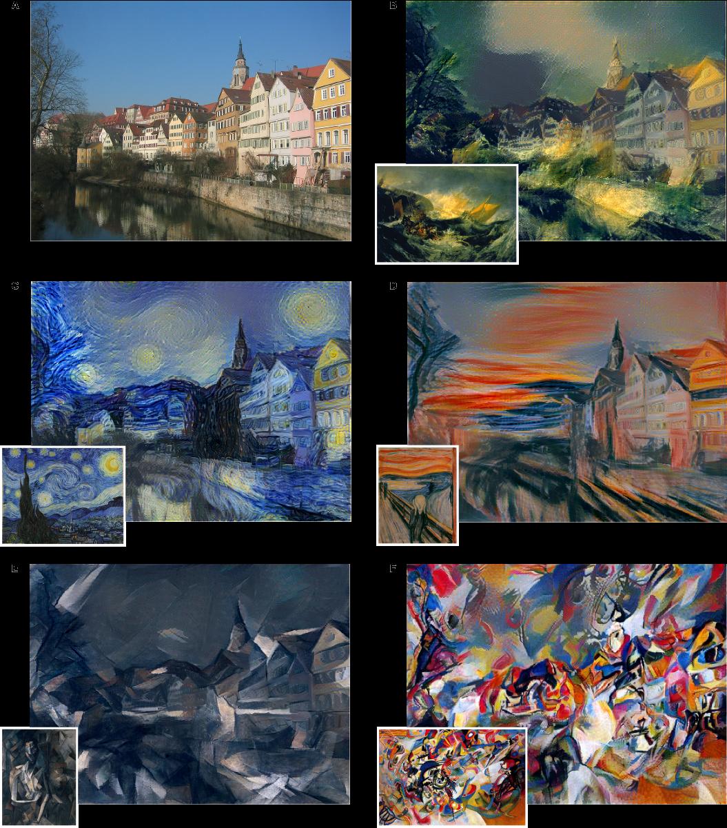
*One example input image with different styles added to it.*
-------------------------
### Rough chapter-wise notes
* Page 1
* A painted image can be decomposed in its content and its artistic style.
* Here they use a neural network to separate content and style from each other (and to apply that style to an existing image).
* Page 2
* Representations get more abstract as you go deeper in networks, hence they should more resemble the actual content (as opposed to the artistic style).
* They call the feature responses in higher layers *content representation*.
* To capture style information, they use a method that was originally designed to capture texture information.
* They somehow build a feature space on top of the existing one, that is somehow dependent on correlations of features. That leads to a "stationary" (?) and multi-scale representation of the style.
* Page 3
* They use VGG as their base CNN.
* Page 4
* Based on the extracted style features, they can generate a new image, which has equal activations in these style features.
* The new image should match the style (texture, color, localized structures) of the artistic image.
* The style features become more and more abtstract with higher layers. They call that multi-scale the *style representation*.
* The key contribution of the paper is a method to separate style and content representation from each other.
* These representations can then be used to change the style of an existing image (by changing it so that its content representation stays the same, but its style representation matches the artwork).
* Page 6
* The generated images look most appealing if all features from the style representation are used. (The lower layers tend to reflect small features, the higher layers tend to reflect larger features.)
* Content and style can't be separated perfectly.
* Their loss function has two terms, one for content matching and one for style matching.
* The terms can be increased/decreased to match content or style more.
* Page 8
* Previous techniques work only on limited or simple domains or used non-parametric approaches (see non-photorealistic rendering).
* Previously neural networks have been used to classify the time period of paintings (based on their style).
* They argue that separating content from style might be useful and many other domains (other than transfering style of paintings to images).
* Page 9
* The style representation is gathered by measuring correlations between activations of neurons.
* They argue that this is somehow similar to what "complex cells" in the primary visual system (V1) do.
* They note that deep convnets seem to automatically learn to separate content from style, probably because it is helpful for style-invariant classification.
* Page 9, Methods
* They use the 19 layer VGG net as their basis.
* They use only its convolutional layers, not the linear ones.
* They use average pooling instead of max pooling, as that produced slightly better results.
* Page 10, Methods
* The information about the image that is contained in layers can be visualized. To do that, extract the features of a layer as the labels, then start with a white noise image and change it via gradient descent until the generated features have minimal distance (MSE) to the extracted features.
* The build a style representation by calculating Gram Matrices for each layer.
* Page 11, Methods
* The Gram Matrix is generated in the following way:
* Convert each filter of a convolutional layer to a 1-dimensional vector.
* For a pair of filters i, j calculate the value in the Gram Matrix by calculating the scalar product of the two vectors of the filters.
* Do that for every pair of filters, generating a matrix of size #filters x #filters. That is the Gram Matrix.
* Again, a white noise image can be changed with gradient descent to match the style of a given image (i.e. minimize MSE between two Gram Matrices).
* That can be extended to match the style of several layers by measuring the MSE of the Gram Matrices of each layer and giving each layer a weighting.
* Page 12, Methods
* To transfer the style of a painting to an existing image, proceed as follows:
* Start with a white noise image.
* Optimize that image with gradient descent so that it minimizes both the content loss (relative to the image) and the style loss (relative to the painting).
* Each distance (content, style) can be weighted to have more or less influence on the loss function.
|
