
|
Welcome to ShortScience.org! |


|
- ShortScience.org is a platform for post-publication discussion aiming to improve accessibility and reproducibility of research ideas.
- The website has 1584 public summaries, mostly in machine learning, written by the community and organized by paper, conference, and year.
- Reading summaries of papers is useful to obtain the perspective and insight of another reader, why they liked or disliked it, and their attempt to demystify complicated sections.
- Also, writing summaries is a good exercise to understand the content of a paper because you are forced to challenge your assumptions when explaining it.
- Finally, you can keep up to date with the flood of research by reading the latest summaries on our Twitter and Facebook pages.
A Neural Algorithm of Artistic Style
Leon A. Gatys and Alexander S. Ecker and Matthias Bethge
arXiv e-Print archive - 2015 via Local arXiv
Keywords: cs.CV, cs.NE, q-bio.NC
First published: 2015/08/26 (8 years ago)
Abstract: In fine art, especially painting, humans have mastered the skill to create unique visual experiences through composing a complex interplay between the content and style of an image. Thus far the algorithmic basis of this process is unknown and there exists no artificial system with similar capabilities. However, in other key areas of visual perception such as object and face recognition near-human performance was recently demonstrated by a class of biologically inspired vision models called Deep Neural Networks. Here we introduce an artificial system based on a Deep Neural Network that creates artistic images of high perceptual quality. The system uses neural representations to separate and recombine content and style of arbitrary images, providing a neural algorithm for the creation of artistic images. Moreover, in light of the striking similarities between performance-optimised artificial neural networks and biological vision, our work offers a path forward to an algorithmic understanding of how humans create and perceive artistic imagery.
more
less
Leon A. Gatys and Alexander S. Ecker and Matthias Bethge
arXiv e-Print archive - 2015 via Local arXiv
Keywords: cs.CV, cs.NE, q-bio.NC
First published: 2015/08/26 (8 years ago)
Abstract: In fine art, especially painting, humans have mastered the skill to create unique visual experiences through composing a complex interplay between the content and style of an image. Thus far the algorithmic basis of this process is unknown and there exists no artificial system with similar capabilities. However, in other key areas of visual perception such as object and face recognition near-human performance was recently demonstrated by a class of biologically inspired vision models called Deep Neural Networks. Here we introduce an artificial system based on a Deep Neural Network that creates artistic images of high perceptual quality. The system uses neural representations to separate and recombine content and style of arbitrary images, providing a neural algorithm for the creation of artistic images. Moreover, in light of the striking similarities between performance-optimised artificial neural networks and biological vision, our work offers a path forward to an algorithmic understanding of how humans create and perceive artistic imagery.


[link]
* The paper describes a method to separate content and style from each other in an image.
* The style can then be transfered to a new image.
* Examples:
* Let a photograph look like a painting of van Gogh.
* Improve a dark beach photo by taking the style from a sunny beach photo.
### How
* They use the pretrained 19-layer VGG net as their base network.
* They assume that two images are provided: One with the *content*, one with the desired *style*.
* They feed the content image through the VGG net and extract the activations of the last convolutional layer. These activations are called the *content representation*.
* They feed the style image through the VGG net and extract the activations of all convolutional layers. They transform each layer to a *Gram Matrix* representation. These Gram Matrices are called the *style representation*.
* How to calculate a *Gram Matrix*:
* Take the activations of a layer. That layer will contain some convolution filters (e.g. 128), each one having its own activations.
* Convert each filter's activations to a (1-dimensional) vector.
* Pick all pairs of filters. Calculate the scalar product of both filter's vectors.
* Add the scalar product result as an entry to a matrix of size `#filters x #filters` (e.g. 128x128).
* Repeat that for every pair to get the Gram Matrix.
* The Gram Matrix roughly represents the *texture* of the image.
* Now you have the content representation (activations of a layer) and the style representation (Gram Matrices).
* Create a new image of the size of the content image. Fill it with random white noise.
* Feed that image through VGG to get its content representation and style representation. (This step will be repeated many times during the image creation.)
* Make changes to the new image using gradient descent to optimize a loss function.
* The loss function has two components:
* The mean squared error between the new image's content representation and the previously extracted content representation.
* The mean squared error between the new image's style representation and the previously extracted style representation.
* Add up both components to get the total loss.
* Give both components a weight to alter for more/less style matching (at the expense of content matching).
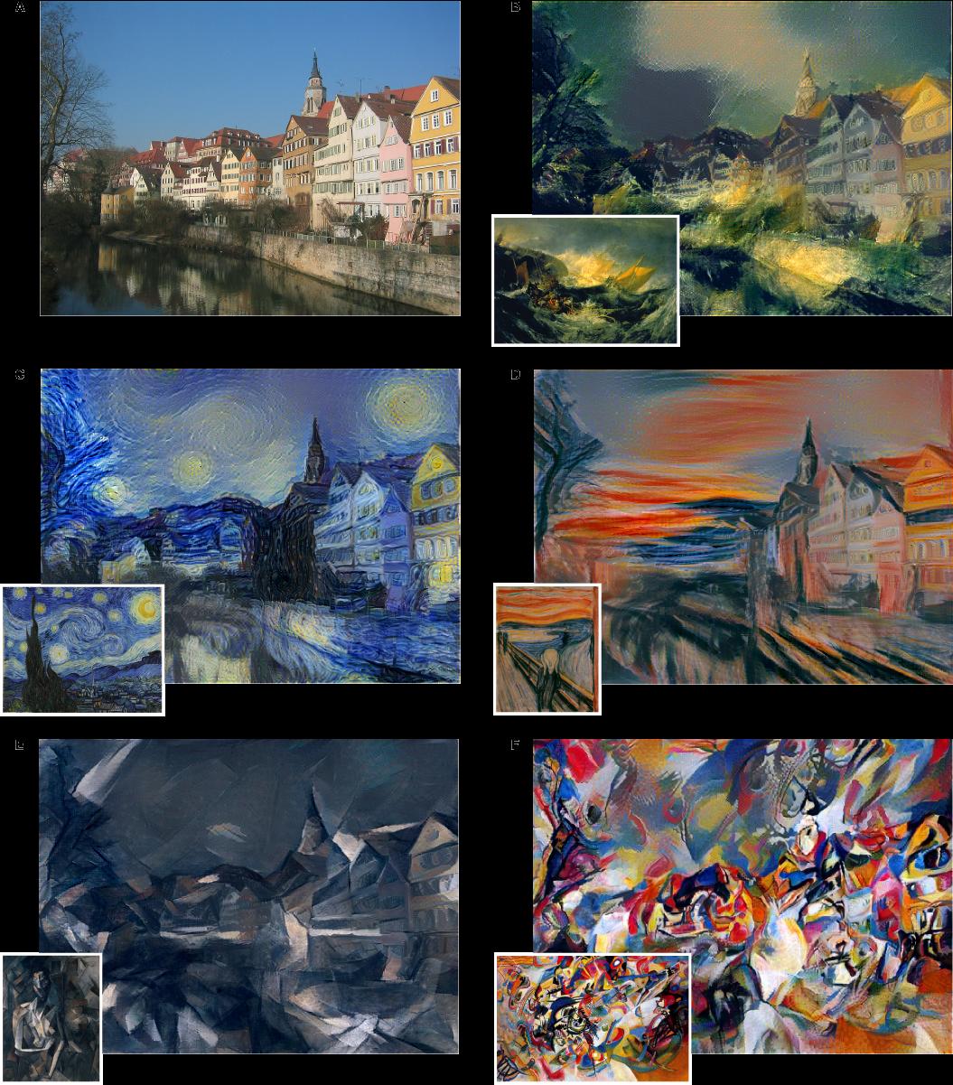
*One example input image with different styles added to it.*
-------------------------
### Rough chapter-wise notes
* Page 1
* A painted image can be decomposed in its content and its artistic style.
* Here they use a neural network to separate content and style from each other (and to apply that style to an existing image).
* Page 2
* Representations get more abstract as you go deeper in networks, hence they should more resemble the actual content (as opposed to the artistic style).
* They call the feature responses in higher layers *content representation*.
* To capture style information, they use a method that was originally designed to capture texture information.
* They somehow build a feature space on top of the existing one, that is somehow dependent on correlations of features. That leads to a "stationary" (?) and multi-scale representation of the style.
* Page 3
* They use VGG as their base CNN.
* Page 4
* Based on the extracted style features, they can generate a new image, which has equal activations in these style features.
* The new image should match the style (texture, color, localized structures) of the artistic image.
* The style features become more and more abtstract with higher layers. They call that multi-scale the *style representation*.
* The key contribution of the paper is a method to separate style and content representation from each other.
* These representations can then be used to change the style of an existing image (by changing it so that its content representation stays the same, but its style representation matches the artwork).
* Page 6
* The generated images look most appealing if all features from the style representation are used. (The lower layers tend to reflect small features, the higher layers tend to reflect larger features.)
* Content and style can't be separated perfectly.
* Their loss function has two terms, one for content matching and one for style matching.
* The terms can be increased/decreased to match content or style more.
* Page 8
* Previous techniques work only on limited or simple domains or used non-parametric approaches (see non-photorealistic rendering).
* Previously neural networks have been used to classify the time period of paintings (based on their style).
* They argue that separating content from style might be useful and many other domains (other than transfering style of paintings to images).
* Page 9
* The style representation is gathered by measuring correlations between activations of neurons.
* They argue that this is somehow similar to what "complex cells" in the primary visual system (V1) do.
* They note that deep convnets seem to automatically learn to separate content from style, probably because it is helpful for style-invariant classification.
* Page 9, Methods
* They use the 19 layer VGG net as their basis.
* They use only its convolutional layers, not the linear ones.
* They use average pooling instead of max pooling, as that produced slightly better results.
* Page 10, Methods
* The information about the image that is contained in layers can be visualized. To do that, extract the features of a layer as the labels, then start with a white noise image and change it via gradient descent until the generated features have minimal distance (MSE) to the extracted features.
* The build a style representation by calculating Gram Matrices for each layer.
* Page 11, Methods
* The Gram Matrix is generated in the following way:
* Convert each filter of a convolutional layer to a 1-dimensional vector.
* For a pair of filters i, j calculate the value in the Gram Matrix by calculating the scalar product of the two vectors of the filters.
* Do that for every pair of filters, generating a matrix of size #filters x #filters. That is the Gram Matrix.
* Again, a white noise image can be changed with gradient descent to match the style of a given image (i.e. minimize MSE between two Gram Matrices).
* That can be extended to match the style of several layers by measuring the MSE of the Gram Matrices of each layer and giving each layer a weighting.
* Page 12, Methods
* To transfer the style of a painting to an existing image, proceed as follows:
* Start with a white noise image.
* Optimize that image with gradient descent so that it minimizes both the content loss (relative to the image) and the style loss (relative to the painting).
* Each distance (content, style) can be weighted to have more or less influence on the loss function.
 |

Deep Adversarial Networks for Biomedical Image Segmentation Utilizing Unannotated Images
Zhang, Yizhe and Yang, Lin and Chen, Jianxu and Fredericksen, Maridel and Hughes, David P. and Chen, Danny Z.
Medical Image Computing and Computer Assisted Interventions Conference - 2017 via Local Bibsonomy
Keywords: dblp
Zhang, Yizhe and Yang, Lin and Chen, Jianxu and Fredericksen, Maridel and Hughes, David P. and Chen, Danny Z.
Medical Image Computing and Computer Assisted Interventions Conference - 2017 via Local Bibsonomy
Keywords: dblp
|
[link]
This work improves the performance of a segmentation network by utilizing unlabelled data. They use a discriminator (they call EN) to distinguish between annotated and unannotated examples. They then train the segmentation generator (they call SN) based on what will fool the discriminator. https://i.imgur.com/7CfKnh5.png Three training phases are shown above This work is really great. They are using the segmentation to condition the discriminator which will learn to point out flaws when applying the segmentation to the unlabelled examples. Then these flaws in the segmentation are corrected by using the gradients from the discriminator to adjust the segmentation. In contrast with other semi-supervised approaches which learn a latent space for all samples, labelled and unlabelled, and then uses this space to learn a classifier or segmentation; this approach looks for the boundaries of the space only. The unlabelled examples are used to bias the representation learned by the segmentation network to conform to the distribution represented by all observed examples. Read this paper for more: https://arxiv.org/abs/1611.08408 Poster: https://i.imgur.com/eR5jgwn.png |

U-Net: Convolutional Networks for Biomedical Image Segmentation
Ronneberger, Olaf and Fischer, Philipp and Brox, Thomas
Medical Image Computing and Computer Assisted Interventions Conference - 2015 via Local Bibsonomy
Keywords: dblp
Ronneberger, Olaf and Fischer, Philipp and Brox, Thomas
Medical Image Computing and Computer Assisted Interventions Conference - 2015 via Local Bibsonomy
Keywords: dblp
|
[link]
1. U-NET learns segmentation in an end to end images.
2. They solved Challenges are
        * Very few annotated images (approx. 30 per application).
        * Touching objects of the same class.
# How:
* Input image is fed in to the network, then the data is propagated through the network along all possible path at the end segmentation maps comes out.
* In U-net architecture, each blue box corresponds to a multi-channel feature map. The number of channels is denoted on top of the box. The x-y-size is provided at the lower left edge of the box. White boxes represent copied feature maps. The arrows denote the different operations.
https://i.imgur.com/Usxmv6r.png
* In two 3x3 convolutions (unpadded convolutions), each followed by a rectified linear unit (ReLU) and a 2x2 max pooling operation with stride 2for down sampling. At each down sampling step they double the number of feature channels.
* Contracting path (left side from up to down) is increases the feature channel and reduces the steps and an expansive path (right side from down to up) consists of sequence of up convolution and concatenation with the corresponds high resolution features from contracting path.
* The network does not have any fully connected layers and only uses the valid part of each convolution, i.e., the segmentation map only contains the pixels, for which the full context is available in the input image.

## Challenges:
1. Overlap-tile strategy for seamless segmentation of arbitrary large images:
     * To predict the pixels in the border region of the image, the missing context is extrapolated by mirroring the input image.
     * In fig, segmentation of the yellow area uses input data of the blue area and the raw data extrapolation by mirroring.
https://i.imgur.com/NUbBRUG.png
2. Augment training data using deformation:
    * They use excessive data augmentation by applying elastic deformations to the available training images.
    * Then the network to learn invariance to such deformations, without the need to see these transformations in the annotated image corpus.
    * Deformation used to be the most common variation in tissue and realistic deformations can be simulated efficiently.
https://i.imgur.com/CyC8Hmd.png
3. Segmentation of touching object of the same class:
    * They propose the use of a weighted loss, where the separating background labels between touching cells obtain a large weight in the loss function.
    * Ensure separation of touching objects, in that segmentation mask for training (inserted background between touching objects) get the loss weights for each pixel.
https://i.imgur.com/ds7psDB.png
4. Segmentation of neural structure in electro-microscopy(EM):
    * Ongoing challenge since ISBI 2012 in this dataset structures with low contrast, fuzzy membranes and other cell components.
    * The training data is a set of 30 images (512x512 pixels) from serial section transmission electron microscopy of the Drosophila first instar larva ventral nerve cord (VNC). Each image comes with corresponding fully annotated ground truth segmentation map for cells(white) and membranes (black).
    * An evaluation can be obtained by sending the predicted membrane probability map to the organizers. The evaluation is done by thresholding  the map at 10 different levels and computation of the warping error, the Rand error and the pixel error.

### Results:
* The u-net (averaged over 7 rotated versions of the input data) achieves with-out any further pre or post-processing a warping error of 0.0003529, a rand-error of 0.0382 and a pixel error of 0.0611.
https://i.imgur.com/6BDrByI.png
* ISBI cell tracking challenge 2015, one of the dataset contains cell phase contrast microscopy has strong shape variations,weak outer borders, strong irrelevant inner borders and cytoplasm has same structure like background.
https://i.imgur.com/vDflYEH.png
* The first data set PHC-U373 contains Glioblastoma-astrocytoma U373 cells on a polyacrylimide substrate recorded by phase contrast microscopy- It contains 35 partially annotated training images. Here we achieve an average IOU ("intersection over union") of 92%,which is significantly better than the second best algorithm with 83%.
https://i.imgur.com/of4rAYP.png
* The second data set DIC-HeLa are HeLa cells on a flat glass recorded by differential interference contrast (DIC) microscopy - It contains 20 partially annotated training images. Here we achieve an average IOU of 77.5% which is significantly better than the second best algorithm with 46%.
https://i.imgur.com/Y9wY6Lc.png
|

Tumor Phylogeny Topology Inference via Deep Learning
Erfan Sadeqi Azer and Mohammad Haghir Ebrahimabadi and Salem Malikić and Roni Khardon and S. Cenk Sahinalp
bioRxiv: The preprint server for biology - 0 via Local CrossRef
Keywords:
Erfan Sadeqi Azer and Mohammad Haghir Ebrahimabadi and Salem Malikić and Roni Khardon and S. Cenk Sahinalp
bioRxiv: The preprint server for biology - 0 via Local CrossRef
Keywords:
|
[link]
A very simple (but impractical) discrete model of subclonal evolution would include the following events:

* Division of a cell to create two cells:
    * **Mutation** at a location in the genome of the new cells
* Cell death at a new timestep
* Cell survival at a new timestep

Because measurements of mutations are usually taken at one time point, this is taken to be at the end of a time series of these events, where a tiny of subset of cells are observed and a **genotype matrix** $A$ is produced, in which mutations and cells are arbitrarily indexed such that $A_{i,j} = 1$ if mutation $j$ exists in cell $i$. What this matrix allows us to see is the proportion of cells which *both have mutation $j$*.

Unfortunately, I don't get to observe $A$, in practice $A$ has been corrupted by IID binary noise to produce $A'$. This paper focuses on difference inference problems given $A'$, including *inferring $A$*, which is referred to as **`noise_elimination`**. The other problems involve inferring only properties of the matrix $A$, which are referred to as:

* **`noise_inference`**: predict whether matrix $A$ would satisfy the *three gametes rule*, which asks if a given genotype matrix *does not describe a branching phylogeny* because a cell has inherited mutations from two different cells (which is usually assumed to be impossible under the infinite sites assumption). This can be computed exactly from $A$.
* **Branching Inference**: it's possible that all mutations are inherited between the cells observed; in which case there are *no branching events*. The paper states that this can be computed by searching over permutations of the rows and columns of $A$. The problem is to predict from $A'$ if this is the case.

In both problems inferring properties of $A$, the authors use fully connected networks with two hidden layers on simulated datasets of matrices. For **`noise_elimination`**, computing $A$ given $A'$, the authors use a network developed for neural machine translation called a [pointer network][pointer]. They also find it necessary to map $A'$ to a matrix $A''$, turning every element in $A'$ to a fixed length row containing the location, mutation status and false positive/false negative rate.

Unfortunately, reported results on real datasets are reported only for branching inference and are limited by the restriction on input dimension. The inferred branching probability reportedly matches that reported in the literature.

[pointer]: https://arxiv.org/abs/1409.0473
|

RIN4 Functions with Plasma Membrane H+-ATPases to Regulate Stomatal Apertures during Pathogen Attack
Jun Liu and James M. Elmore and Anja T. Fuglsang and Michael G. Palmgren and Brian J. Staskawicz and Gitta Coaker
PLoS Biology - 2009 via Local CrossRef
Keywords:
Jun Liu and James M. Elmore and Anja T. Fuglsang and Michael G. Palmgren and Brian J. Staskawicz and Gitta Coaker
PLoS Biology - 2009 via Local CrossRef
Keywords:
|
[link]
Pathogen perception by the plant innate immune system is of central importance to plant survival and productivity. The Arabidopsis protein RIN4 is a negative regulator of plant immunity. In order to identify additional proteins involved in RIN4-mediated immune signal transduction, we purified components of the RIN4 protein complex. We identified six novel proteins that had not previously been implicated in RIN4 signaling, including the plasma membrane (PM) H+-ATPases AHA1 and/or AHA2. RIN4 interacts with AHA1 and AHA2 both in vitro and in vivo. RIN4 overexpression and knockout lines exhibit differential PM H+-ATPase activity. PM H+-ATPase activation induces stomatal opening, enabling bacteria to gain entry into the plant leaf; inactivation induces stomatal closure thus restricting bacterial invasion. The rin4 knockout line exhibited reduced PM H+-ATPase activity and, importantly, its stomata could not be re-opened by virulent Pseudomonas syringae. We also demonstrate that RIN4 is expressed in guard cells, highlighting the importance of this cell type in innate immunity. These results indicate that the Arabidopsis protein RIN4 functions with the PM H+-ATPase to regulate stomatal apertures, inhibiting the entry of bacterial pathogens into the plant leaf during infection. Author Summary Top Plants are continuously exposed to microorganisms. In order to resist infection, plants rely on their innate immune system to inhibit both pathogen entry and multiplication. We investigated the function of the Arabidopsis protein RIN4, which acts as a negative regulator of plant innate immunity. We biochemically identified six novel RIN4-associated proteins and characterized the association between RIN4 and the plasma membrane H+-ATPase pump. Our results indicate that RIN4 functions in concert with this pump to regulate leaf stomata during the innate immune response, when stomata close to block the entry of bacterial pathogens into the leaf interior. |
